An Introduction To Transfer Learning With Exercises

At the end of this lesson, you will be able to use transfer learning to build highly accurate computer vision models for your custom purposes, even when you have relatively little data.
Ayush Chaurasia
Created on June 14|Last edited on June 14
Comment
This article is an expansion of Kaggle's course on Transfer Learning. We expand on the original content (included) with additional context and visualizations.
﻿
﻿
Lesson
﻿
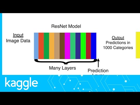
Sample CodeSpecify Model
from tensorflow.python.keras.applications import ResNet50
from tensorflow.python.keras.models import Sequential
from tensorflow.python.keras.layers import Dense, Flatten, GlobalAveragePooling2D
﻿
num_classes = 2
resnet_weights_path = '../input/resnet50/resnet50_weights_tf_dim_ordering_tf_kernels_notop.h5'
﻿
my_new_model = Sequential()
my_new_model.add(ResNet50(include_top=False, pooling='avg', weights=resnet_weights_path))
my_new_model.add(Dense(num_classes, activation='softmax'))
﻿
# Say not to train first layer (ResNet) model. It is already trained
my_new_model.layers[0].trainable = False
Compile Model
my_new_model.compile(optimizer='sgd', loss='categorical_crossentropy', metrics=['accuracy'])
Fit Model
from tensorflow.python.keras.applications.resnet50 import preprocess_input
from tensorflow.python.keras.preprocessing.image import ImageDataGenerator
﻿
image_size = 224
data_generator = ImageDataGenerator(preprocessing_function=preprocess_input)
﻿
﻿
train_generator = data_generator.flow_from_directory(
        '../input/urban-and-rural-photos/rural_and_urban_photos/train',
        target_size=(image_size, image_size),
        batch_size=24,
        class_mode='categorical')
﻿
validation_generator = data_generator.flow_from_directory(
        '../input/urban-and-rural-photos/rural_and_urban_photos/val',
        target_size=(image_size, image_size),
        class_mode='categorical')
﻿
my_new_model.fit_generator(
        train_generator,
        steps_per_epoch=3,
        validation_data=validation_generator,
        validation_steps=1)
Found 72 images belonging to 2 classes.
Found 20 images belonging to 2 classes.
Epoch 1/1
3/3 [==============================] - 21s 7s/step - loss: 0.5654 
- acc: 0.7361 - val_loss: 0.4350 - val_acc: 0.8500
<tensorflow.python.keras.callbacks.History at 0x7f5f8793fb70>
Note on Results:
The printed validation accuracy can be meaningfully better than the training accuracy at this stage. This can be puzzling at first.
It occurs because the training accuracy was calculated at multiple points as the network was improving (the numbers in the convolutions were being updated to make the model more accurate). The network was inaccurate when the model saw the first training images, since the weights hadn't been trained/improved much yet. Those first training results were averaged into the measure above.
The validation loss and accuracy measures were calculated after the model had gone through all the data. So the network had been fully trained when these scores were calculated.
This isn't a serious issue in practice, and we tend not to worry about it.
IntroductionThe cameraman who shot our deep learning videos mentioned a problem that we can solve with deep learning.
He offers a service that scans photographs to store them digitally. He uses a machine that quickly scans many photos. But depending on the orientation of the original photo, many images are digitized sideways. He fixes these manually, looking at each photo to determine which ones to rotate.
In this exercise, you will build a model that distinguishes which photos are sideways and which are upright, so an app could automatically rotate each image if necessary.
If you were going to sell this service commercially, you might use a large dataset to train the model. But you'll have great success with even a small dataset. You'll work with a small dataset of dog pictures, half of which are rotated sideways.
Specifying and compiling the model look the same as in the example you've seen. But you'll need to make some changes to fit the model.
1) Specify the ModelSince this is your first time, we'll provide some starter code for you to modify. You will probably copy and modify code the first few times you work on your own projects.
from tensorflow.keras.applications import ResNet50
from tensorflow.keras.models import Sequential
from tensorflow.keras.layers import Dense, Flatten, GlobalAveragePooling2D
﻿
num_classes = 2
resnet_weights_path = '../input/resnet50/resnet50_weights_tf_dim_ordering_tf_kernels_notop.h5'
﻿
my_new_model = Sequential()
my_new_model.add(ResNet50(include_top=False, pooling='avg', weights=resnet_weights_path))
my_new_model.add(Dense(num_classes, activation='softmax'))
﻿
# Indicate whether the first layer should be trained/changed or not.
my_new_model.layers[0].trainable = False
2) Compile the ModelYou now compile the model with the following line. Run this cell.
my_new_model.compile(optimizer='sgd', 
                     loss='categorical_crossentropy', 
                     metrics=['accuracy'])
The compile model doesn't change the values in any convolutions. In fact, your model has not even received an argument with data yet. Compile specifies how your model will make updates a later fit step where it receives data. That is the part that will take longer.
3) Review the Compile StepYou provided three arguments in the compile step.
optimizer
loss
metrics
4) Train FunctionYour training data is in the directory ../input/dogs-gone-sideways/images/train. The validation data is in ../input/dogs-gone-sideways/images/val. Use that information when setting up train_generator and validation_generator.
You have 220 images of training data and 217 of validation data.  For the training generator, we set a batch size of 10. Figure out the appropriate value of steps_per_epoch in your fit_generator call. Using WandbCallback will autpmatically log the metrics being optimized to the dashboard.
from tensorflow.keras.applications.resnet50 import preprocess_input
from tensorflow.keras.preprocessing.image import ImageDataGenerator
import wandb
from wandb.keras import WandbCallback
def train(model):
    wandb.init(project='Kaggle-DL')
    image_size = 224
    data_generator = ImageDataGenerator(preprocess_input)
﻿
    train_generator = data_generator.flow_from_directory(
                                            directory='../input/dogs-gone-sideways/images/train',
                                            target_size=(image_size, image_size),
                                            batch_size=10,
                                            class_mode='categorical')
﻿
    validation_generator = data_generator.flow_from_directory(
                                            directory="../input/dogs-gone-sideways/images/val",
                                            target_size=(image_size, image_size),
                                            class_mode='categorical')
﻿
    # fit_stats below saves some statistics describing how model fitting went
    # the key role of the following line is how it changes my_new_model by fitting to data
    fit_stats = model.fit_generator(train_generator,
                                           steps_per_epoch=22,
                                           validation_data=validation_generator,
                                           validation_steps=1,
                                           epochs = 10,
                                            callbacks=[WandbCallback()]
                                          )
﻿
5) Compare OptimizersNow let us clone the model that we've created and compile the models using different optimizers to see how they perform on the same dataset. We've already built our train function to log the metrics automatically which will facilitate this comparison.
from tensorflow.keras.models import clone_model
﻿
model1 = Sequential()
model1.add(ResNet50(include_top=False, pooling='avg', weights=resnet_weights_path))
model1.add(Dense(num_classes, activation='softmax'))
﻿
# Indicate whether the first layer should be trained/changed or not.
model1.layers[0].trainable = False
model2 =clone_model(model1)
﻿
model1.compile(optimizer='sgd', 
                     loss='categorical_crossentropy', 
                     metrics=['accuracy'])
model2.compile(optimizer='adam', 
                     loss='categorical_crossentropy', 
                     metrics=['accuracy'])
train(model1)
train(model2)
﻿
6) VisualizationsLet's take a look at the metrics logged by  WandbCallback and compare the performance for our models
LossIt is clear from the plots generated on the right that the Adam optimizer converges much faster than the sgd optimizer on this particular model and dataset
﻿
﻿
﻿
AccuracyAs expected from the loss plot,  the model compiled with `Adam` optimizer has much larger train as well as validation accuracy than the one compiled with `SGD` optimizer
﻿
﻿
Usage Metrics In addition to optimization metrics, `WandbCallback` aslo logs the system usage metrics. GPU metrics are the most important usage metrics when is comes to kaggle kernels as you get limited free GPU hours per month.
﻿
﻿
﻿
Keep GoingMove on to learn about data augmentation. It is a clever and easy way to improve your models. Then you'll apply data augmentation to this automatic image rotation problem.
﻿
Add a comment