실시간 사회적 거리두기 감지기
이 보고서는 실시간 비디오 피드를 활용해 온디바이스 추론을 수행하는 빠르고 정확한 사회적 거리 감지기를 구축하는 방법을 설명합니다. 이 글은 AI 번역본입니다. 오역이 있을 수 있으니 댓글로 알려주세요.
Created on September 15|Last edited on September 15
Comment
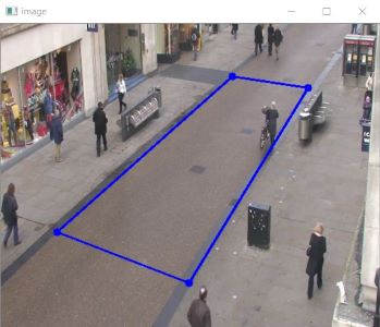
소개
Colab 노트북을 확인하세요
질병이 신체 접촉을 통해 전파되는 모든 팬데믹 상황에서 사회적 거리두기는 질병 확산을 억제하는 가장 효과적인 방법입니다. 특히 최근 코로나19가 많은 사람들의 삶을 파괴한 상황에서, 사회적 거리를 유지하는 것은 필수적입니다. 이에 따라 다수의 산업 분야에서는 사람들이 이 안전 수칙을 얼마나 준수하고 있는지 파악할 수 있는 도구를 요구하고 있습니다.
사회적 거리 감지기는 이러한 상황을 해결하는 한 가지 방법입니다.
접근 방법
이 목적을 달성하기 위해 파이프라인은 세 가지 핵심 측면으로 구성됩니다:
- 실시간 보행자 감지: 객체 감지는 객체 분류와 객체 위치 추정의 결합입니다. 이 방법은 여러 객체 클래스의 존재와 위치를 탐지하도록 학습됩니다. 여기서 우리가 다루는 객체는 ‘사람’입니다. 실시간 비디오 피드에서 사람 클래스를 충분한 신뢰도로 식별해야 합니다. 객체 감지에는 다양한 접근법이 있으며, 다음과 같을 수 있습니다 Region Classification Method R-CNN 또는 Fast R-CNN과 함께," Implicit Anchor Method Faster R-CNN, YOLO v1–v4, 또는 EfficientDet와 함께, Keypoint Estimation Method CenterNet 또는 CornerNet과 함께.
우리의 목표는 장면에서 보행자를 탐지하고 그 좌표를 찾아내는 것입니다. 온디바이스 추론을 위해 우리는 사용할 예정입니다. SSD(Single Shot Detector) 모델입니다. 이 모델은 TensorFlow Lite로 변환될 예정이며, TensorFlow Lite 객체 감지 API(TFOD)여기에서 사용하는 모바일 모델은 SSD_MobileDet_cpu_coco.
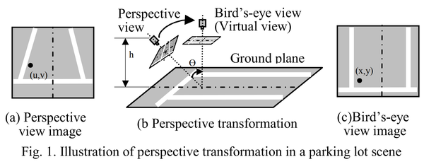
- 보정: 각 프레임은 임의의 원근 시점을 가지므로 사람들 사이의 상대 거리를 일관되게 분석하거나 계산하기 어렵습니다. 따라서 프레임을 버드아이(탑다운) 뷰로 변환하는 과정이 필요합니다. 이 과정을 보정이라고 합니다. 이를 통해 모든 사람이 동일한 평평한 지면 평면 위에 놓이도록 보장합니다. 이는 Social-distance Detector를 개선하고 파이프라인의 최종 단계에서 정확한 측정을 얻기 위한 단계입니다.
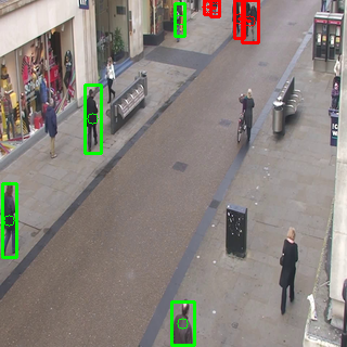
- 사회적 거리 위반 판별: 이제 버드아이(탑다운) 뷰에서 사람들의 위치를 얻었으므로, 파이프라인의 마지막 단계는 어떤 사람이 한 명 이상과 과도하게 가까운지 확인하는 것입니다. 기준을 준수하는 사람은 녹색 바운딩 박스로 표시하고, 위반자는 두 개 이상의 연결선과 함께 빨간색 박스로 강조합니다.
다음 내용을 다룹니다:
- TensorFlow Lite와 MobileDet
- 모델 변환
- MobileDet 변형 모델 벤치마크
- 보정과 변환
- 사회적 거리 위반 판별
- 시각화
- 추론
- 결론
TensorFlow Lite와 MobileDet
온디바이스 추론 이야기로 돌아가면, MobileDet 가장 적합합니다. COCO 객체 탐지 과제에서 MobileDet은 유사한 모바일 CPU 추론 지연에서 MobileNetV3+SSDLite보다 mAP 1.7만큼 더 우수한 성능을 보입니다. 또한 모바일 CPU에서 MobileDet은 MobileNetV2+SSDLite보다 mAP 1.9만큼 앞섭니다. 더 자세한 내용은 여기에서 MobileDet
이 모델을 TensorFlow Lite로 변환하는 목적은 낮은 지연 시간과 작은 바이너리 크기로 온디바이스 머신러닝 추론을 가능하게 하기 위함입니다. TensorFlow Lite는 개발자가 모바일, 임베디드, IoT 기기에서 TensorFlow 모델을 실행할 수 있도록 설계되었습니다. 더 알아보려면 여기에서 TensorFlow Lite
SSD(Single Shot Detector) 모델은 이미지를 입력으로 받습니다. 예를 들어 입력 이미지가 300 × 300 픽셀이고 각 픽셀에 빨강, 파랑, 초록의 3개 채널이 있다고 하면, 이 이미지는 모델에 270,000바이트(300 × 300 × 3)의 평탄화된 버퍼로 전달됩니다. 모델이 양자화되어 있다면 각 값은 0에서 255 사이의 값을 나타내는 1바이트여야 합니다. 이 모델은 4개의 배열(위치, 클래스, 신뢰도, 탐지 개수)을 출력합니다. 이 모델을 TensorFlow Lite로 변환하려면, 먼저 TensorFlow Lite 연산자 집합과 호환되는 동결 그래프를 생성해야 합니다(여기에서 설명한 대로 - TF1 또는 TF2). 두 개의 스크립트(TF1 그리고 TF2) 모델 그래프에 최적화된 후처리를 추가합니다. 이 모델 그래프는 이후 양자화를 거쳐 TensorFlow Lite 모델 파일로 변환됩니다. .tflite 세 가지 양자화 과정을 포함한 확장 기능.
- 동적 범위 양자화
- Float16 양자화
- 완전 정수 양자화
모델 변환
이것이 모델입니다. SSD_MobileDet_cpu_coco 우리는 이 모델을 미리 양자화할 예정이다. 이 모델 번들을 압축 해제하면 다음 파일들이 제공된다: 사전 학습된 체크포인트, TensorFlow Lite(TFLite) 호환 모델 그래프, TFLite 모델 파일, 구성 파일, 그리고 그래프 프로토. 모델들은 COCO 데이터셋으로 사전 학습되었다. model.ckpt-* 파일들은 COCO 데이터셋으로 사전 학습된 체크포인트입니다. The tflite_graph.pb 파일은 TFLite 연산자 집합과 호환되는 동결된 추론 그래프로, 사전 학습된 모델 체크포인트에서 내보낸 것입니다. model.tflite 파일은 에서 변환된 TFLite 모델입니다. tflite_graph.pb 동결 그래프.
--- model.ckpt-400000.data-00000-of-00001--- model.ckpt-400000.index--- model.ckpt-400000.meta--- model.tflite--- pipeline.config--- tflite_graph.pb--- tflite_graph.pbtxt
동적 범위 양자화
converter = tf.compat.v1.lite.TFLiteConverter.from_frozen_graph(graph_def_file=model_to_be_quantized,input_arrays=['normalized_input_image_tensor'],output_arrays=['TFLite_Detection_PostProcess','TFLite_Detection_PostProcess:1','TFLite_Detection_PostProcess:2','TFLite_Detection_PostProcess:3'],input_shapes={'normalized_input_image_tensor': [1, 320, 320, 3]})converter.allow_custom_ops = Trueconverter.optimizations = [tf.lite.Optimize.DEFAULT]tflite_model = converter.convert()
이 dynamic range 가중치를 부동소수점에서 정수로 양자화하며, 정밀도는 8비트입니다. 추론 시에는 가중치를 8비트 정밀도에서 부동소수점으로 변환한 뒤 부동소수점 커널로 계산합니다. 위의 코드 블록에서는 다음을 제공해야 합니다. tflite_graph.pb 대신 사용할 파일 model_to_be_quantized. 이 모델은 320 × 320픽셀 크기의 입력 이미지를 받으므로, the input_arrays 그리고 input_shapes 그에 따라 설정됩니다. The output_arrays 네 가지 배열을 출력하도록 설정됩니다: 바운딩 박스 위치, 감지된 객체의 클래스, 신뢰도, 감지 수. 이는 이에 따라 설정됩니다. 가이드
양자화 후 모델 크기는 4.9 MB입니다.
Float16 양자화
converter = tf.compat.v1.lite.TFLiteConverter.from_frozen_graph(graph_def_file=model_to_be_quantized,input_arrays=['normalized_input_image_tensor'],output_arrays=['TFLite_Detection_PostProcess','TFLite_Detection_PostProcess:1','TFLite_Detection_PostProcess:2','TFLite_Detection_PostProcess:3'],input_shapes={'normalized_input_image_tensor': [1, 320, 320, 3]})converter.allow_custom_ops = Trueconverter.target_spec.supported_types = [tf.float16]converter.optimizations = [tf.lite.Optimize.DEFAULT]tflite_model = converter.convert()
이 float 16 양자화를 적용하면 정확도 손실을 거의 일으키지 않으면서 모델 크기가 절반으로 줄어듭니다. 이 방법은 모델의 가중치와 바이어스를 전체 정밀도의 부동소수점(32비트)에서 정밀도가 낮은 부동소수점 데이터 타입(IEEE FP16)으로 양자화합니다. 이전 코드에 한 줄만 추가하면 됩니다. dynamic range 코드 블록: converter.target_spec.supported_types = [tf.float16]
양자화 후 모델 크기는 8.2 MB입니다.
풀 인티저 양자화
converter = tf.compat.v1.lite.TFLiteConverter.from_frozen_graph(graph_def_file=model_to_be_quantized,input_arrays=['normalized_input_image_tensor'],output_arrays=['TFLite_Detection_PostProcess','TFLite_Detection_PostProcess:1','TFLite_Detection_PostProcess:2','TFLite_Detection_PostProcess:3'],input_shapes={'normalized_input_image_tensor': [1, 320, 320, 3]})converter.allow_custom_ops = Trueconverter.representative_dataset = representative_dataset_genconverter.inference_input_type = tf.uint8converter.quantized_input_stats = {"normalized_input_image_tensor": (128, 128)}converter.optimizations = [tf.lite.Optimize.DEFAULT]tflite_model = converter.convert()
풀 인티저 양자화 방법을 사용하려면, 우리는 다음을 사용해야 합니다 representative dataset자체 데이터세트를 만들려면 다음 자료를 참고하세요 여기대표 데이터세트를 생성하는 함수는 다음과 같습니다 여기이 데이터세트는 학습 또는 검증 데이터에서 약 100~150개 샘플로 이루어진 작은 부분집합이면 됩니다. 대표 데이터세트는 소수의 추론 사이클을 실행하여 모델 입력, 활성화(중간 레이어의 출력), 모델 출력을 비롯한 가변 텐서를 보정하는 데 필요합니다.
양자화 후 모델 크기는 4.9 MB입니다.
MobileDet 변형 모델 벤치마크
모델 벤치마크는 목적에 가장 적합한 모델을 선택하는 방법입니다. 한 가지 방법은 각 모델의 지표를 살펴보고 비교하는 것입니다. FPS 그리고 Elapsed Time다음은 제가 기록한 일부 모델 벤치마크입니다:
| Model Name | Model Size(MB) | Elapsed Time(s) | FPS |
|---|---|---|---|
| SSD_mobileDet_cpu_coco_int8 | 4.9 | 705.32 | 0.75 |
| SSD_mobileDet_cpu_coco_fp16 | 8.2 | 52.79 | 10.06 |
| SSD_mobileDet_cpu_coco_dr | 4.9 | 708.57 | 0.75 |
또 다른 방법은 …을 사용하는 것입니다 TensorFlow Lite 벤치마크 도구. 설정해야 합니다 Android 디버그 브리지(adb) 노트북에서 TensorFlow Lite 벤치마크 도구를 사용하려면 안드로이드 기기를 연결하여 모델의 추론 속도를 확인하세요. 저는 오직 fp16 세 가지 변형 중 가장 빠르기 때문에 이것 하나를 사용했습니다.
- 아래 이미지의 첫 번째 결과는 CPU를 스레드 4개로 사용했을 때의 값입니다.
- 아래 이미지의 두 번째 결과는 GPU를 사용했을 때의 값입니다.

캘리브레이션
절차는 다음과 같습니다:
1. 사각형 찾기 - 네 개의 코너 점
이미지 프레임을 원근 시점에서 탑다운(버드아이) 뷰로 변환하려면, 프레임을 왜곡할 사각형의 올바른 좌표를 선택해야 합니다. 이를 위해 차선, 바닥, 지면 등을 기준 대상으로 사용할 수 있습니다.
캘리브레이션은 이미지의 배경만을 기준으로 수행됩니다. 따라서 배경 뷰가 바뀌면 사각형 꼭짓점 좌표도 달라지고, 이에 따라 보정을 위한 변환 행렬 역시 변경됩니다.
카메라 위치와 배경이 고정되어 있다고 가정하면, 전처리 단계에서 지면(도로 또는 바닥) 위의 네 개 코너 포인트를 찾는 것이 가장 쉽습니다. 현재는 사용자 상호작용형 마우스 클릭으로 이를 수행했습니다. mouse_click_event.py 사용자가 코너를 드래그해 사각형을 선택할 수 있도록 합니다.
2. 변환 행렬(M)
보정의 핵심은 변환 행렬입니다.
선택한 코너 포인트를 가져온 뒤 좌표를 올바른 순서로 정렬하고, OpenCV의 getPerspectiveTransform()을 적용하여 변환 행렬(M)을 구합니다.
전체 이미지 프레임을 워핑하려면 다음 매핑 함수를 사용하세요:

여기서 (x, y)는 원본 이미지 좌표를 의미합니다.
이 함수를 사용해 이미지의 코너 포인트(마우스로 클릭한 포인트가 아님)를 매핑하고, 탑다운 뷰에서의 대응 좌표를 얻으세요. 그런 다음 워핑된 프레임에서 좌·우·상·하의 극값 좌표를 계산하고, 이를 이용해 최종 변환 행렬 M을 구합니다.
def getmap(image):# image : first frame of the input videoglobal grid_H, grid_Wh,w=image.shape[:2]# 4 corner points of image are set by default# User needs to finalise the corner points of a road or floor by dragging and dropping the corners#corners=mouse_click_event.adjust_coor_quad(image,corners)corners=[(308, 67), (413, 91), (245, 351), (75, 270)]corners=np.array(corners,dtype="float32")src=order_points(corners)(tl,tr,br,bl)=srcwidth1=np.sqrt(((br[0]-bl[0])**2)+((br[1]-bl[1])**2))width2=np.sqrt(((tr[0]-tl[0])**2)+((tr[1]-tl[1])**2))width=max(int(width1),int(width2))height1=np.sqrt(((tr[0]-br[0])**2)+((tr[1]-br[1])**2))height2=np.sqrt(((tl[0]-bl[0])**2)+((tl[1]-bl[1])**2))height=max(int(height1),int(height2))width=int(width)height=int(height)dest=np.array([[0,0],[width-1,0],[width-1,height-1],[0,height-1]],dtype="float32")M=cv2.getPerspectiveTransform(src,dest)corners=np.array([[0,h-1,1],[w-1,h-1,1],[w-1,0,1],[0,0,1]],dtype="int")warped_corners=np.dot(corners,M.T)warped_corners=warped_corners/warped_corners[:,2].reshape((len(corners),1))warped_corners=np.int64(warped_corners)warped_corners=warped_corners[:,:2]min_coor=np.min(warped_corners,axis=0)max_coor=np.max(warped_corners,axis=0)grid_W,grid_H=max_coor-min_coordest=np.array([[abs(min_coor[0]),abs(min_coor[1])],[abs(min_coor[0])+grid_W-1,abs(min_coor[1])],[abs(min_coor[0])+grid_W-1,abs(min_coor[1])+grid_H-1],[abs(min_coor[0]),abs(min_coor[1])+grid_H-1]],dtype="float32")M=cv2.getPerspectiveTransform(src,dest)return M
앞서 설명했듯이, getmap()은 전처리 단계에서 한 번만 호출하여 변환 행렬을 얻고 각 프레임의 포인트를 보정해야 합니다.
3. 보정
변환 행렬을 사용해 다음을 수행해야 합니다:
- 워핑된 이미지, 즉 버드아이 뷰 그리드에서 검출된 사람들의 위치를 대응하는 위치로 보정합니다.
- 유지해야 할 최소 사회적 거리(MIN_DISTANCE)를 계산합니다.
사람의 평균 신장은 약 5~6피트이며, 사회적 거리는 6피트를 유지해야 합니다. 따라서 보행자 검출 결과에서 사람들의 신장 중앙값을 구해 이를 MIN_DISTANCE로 설정합니다. 다만 거리 위반 판정을 위해 이 값을 사용하려면, 탑다운 뷰를 기준으로 완전히 이루어지므로 이 신장 값을 보정해야 합니다.
def calibration(M,results):# calculate minimum distance for social distancingglobal MIN_DISTANCErect=np.array([r[1] for r in results])h=np.median(rect[:,2]-rect[:,0])coor=np.array([[50,100,1],[50,100+h,1]],dtype="int")coor=np.dot(coor,M.T)coor=coor/coor[:,2].reshape((2,1))coor=np.int64(coor[:,:2])MIN_DISTANCE=int(round(dist.pdist(coor)[0]))#calculate centroid points of detected people location corresponding to bird's eye view black gridcentroids=np.array([r[2] for r in results])centroids=np.c_[centroids,np.ones((centroids.shape[0],1),dtype="int")]warped_centroids=np.dot(centroids,M.T)warped_centroids=warped_centroids/warped_centroids[:,2].reshape((len(centroids),1))warped_centroids=np.int64(warped_centroids)return warped_centroids[:,:2]

사회적 거리 위반 판정
사람들 사이의 거리를 계산하려면, 가능한 모든 쌍의 유클리드 거리를 구해 임계값을 넘는 쌍을 판정하는 브루트포스 방법을 사용할 수 있습니다. 이는 고성능의 파이썬 라이브러리인 numpy와 SciPy를 활용해 쉽게 구현할 수 있습니다. 이거 한번 확인해봐 주세요 자세히 알아보기.
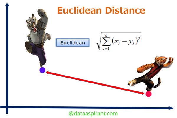
def calc_dist(centroids):# centroids : updated centroids in top-down view coordinatesif len(centroids)<2: # no pair of people, no violationreturn list()# evaluate the pairwise distances between peoplecondensed_dist=dist.pdist(centroids)D=dist.squareform(condensed_dist)locations=np.where(D<MIN_DISTANCE)violate=list(zip(locations[0],locations[1]))violate=np.sort(violate,axis=1)violate=np.unique(violate,axis=0)violate=np.asarray(list(filter(lambda x:x[0]!=x[1],violate)))return violate
시각화
무슨 일이 벌어지는지 시각화하지 않으면 모든 것이 무의미합니다!
우리 프로젝트에서 초록색은 사회적 거리를 준수하는 사람을, 빨간색은 안전 수칙을 위반하는 사람을 의미합니다.
기본적으로 다음과 같은 프레임을 시각화에 사용합니다:
- 출력 - 입력 비디오 프레임과 함께 사람 주위에 초록색과 빨간색 바운딩 박스를 표시합니다. 이해를 돕기 위해 위반자들 사이를 연결하는 빨간 선도 함께 표시합니다.
- 버즈아이 뷰 격자 — 상단에서 내려다본 화면에 검은 프레임을 표시하고, 사람들을 색상 코드(초록/빨강)의 점으로 나타냅니다. 점(즉, 사람)들이 서로 가까워지면 해당 점들 사이에 하나 이상의 빨간 선을 연결해 표시합니다.
- 워프된 이미지 - (선택 사항, 동작 이해용) 입력 비디오 프레임을 상단에서 내려다본 뷰로 보여 주며, 사람 위치를 색상 코드가 적용된 점으로 표시합니다.
출력 프레임 시각화하기
보행자 감지기의 결과는 사람의 위치를 파악하는 데 도움이 됩니다. 위반자 목록은 사람들을 두 개의 범주로 구분하는 데 도움이 됩니다. 지정된 규칙에 따라 색상을 선택해 바운딩 박스를 그리세요.
def visualise_main(frame,results,violate):for (i,(prob,bbox,centroid)) in enumerate(results):(startX,startY,endX,endY)=bbox(cX,cY)=centroidcolour=(0,255,0)if i in np.unique(violate):colour=(0,0,255)frame=cv2.rectangle(frame,(startX,startY),(endX,endY),colour,2)frame=cv2.circle(frame,(cX,cY),5,colour,1)#Drawing the connecting lines between violatorsfor i,j in violate:frame=cv2.line(frame,results[i][2],results[j][2],(0,0,255),2)return frame
버즈아이 뷰 격자와 워프된 프레임 시각화하기
cv2.warpPerspective()를 사용해 메인 프레임의 보정된 워프 이미지를 얻습니다.

보정된 데이터에서 버즈아이 뷰로 사람들의 위치를 찾아 검은 격자 위에 점선 형태의 점으로 표시하세요. 색상은 위반자 목록에 따라 지정합니다. 모든 위반자 쌍 사이에는 빨간 선을 그립니다.

def visualise_grid(image,M,centroids,violate):warped=cv2.warpPerspective(image,M,(grid_W,grid_H),cv2.INTER_AREA, borderMode=cv2.BORDER_CONSTANT, borderValue=(0,0,0))grid=np.zeros(warped.shape,dtype=np.uint8)for i in range(len(centroids)):colour=(0,255,0)if i in np.unique(violate):colour=(0,0,255)grid=cv2.circle(grid,tuple(centroids[i,:]),5,colour,-1)warped=cv2.circle(warped,tuple(centroids[i,:]),5,colour,-1)for i,j in violate:grid=cv2.line(grid,tuple(centroids[i]),tuple(centroids[j]),(0,0,255),2)#cv2_imshow("Bird's eye view grid",cv2.resize(grid,image.shape[:2][::-1]))#cv2_imshow("warped",cv2.resize(warped,image.shape[:2][::-1]))grid=cv2.resize(grid,image.shape[:2][::-1])warped=cv2.resize(warped,image.shape[:2][::-1])return grid,warped
추론
온디바이스에서 TensorFlow Lite 모델을 실행하여 입력 데이터에 기반해 예측을 수행하려면, 이 과정은 추론. 추론을 수행하려면 인터프리터를 통해 모델을 실행해야 합니다. TensorFlow Lite 추론은 아래 단계들을 따라 진행됩니다:
모델 불러오기
처럼 SSD_MobileDet_cpu_coco_fp16 셋 중 가장 좋은 결과를 보였으므로, 이 모델을 불러와 계속 진행하겠습니다. The tf.lite.Interpreter 를 입력으로 받아 .tflite 모델 파일입니다. 텐서는 할당되고, 모델 입력 형상은 다음에서 정의됩니다 HEIGHT, WIDTH.
tflite_model = "ssd_mobiledet_cpu_coco_fp16.tflite"interpreter = tf.lite.Interpreter(model_path=tflite_model)interpreter.allocate_tensors()_, HEIGHT, WIDTH, _ = interpreter.get_input_details()[0]['shape']
입력 텐서 설정
아래 코드 블록은 모델의 모든 입력 세부 정보를 반환합니다.
def set_input_tensor(interpreter, image):tensor_index = interpreter.get_input_details()[0]['index']input_tensor = interpreter.tensor(tensor_index)()[0]input_tensor[:, :] = image
출력 텐서 가져오기
아래 코드 블록은 모든 출력 세부 정보를 반환합니다: Location of Bounding Box, Class, Confidence, Number of detection.
def get_output_tensor(interpreter, index):output_details = interpreter.get_output_details()[index]tensor = np.squeeze(interpreter.get_tensor(output_details['index']))return tensor
보행자 탐지
def pedestrian_detector(interpreter, image, threshold):"""Returns a list of detection results, each as a tuple of object info."""H,W=HEIGHT,WIDTHset_input_tensor(interpreter, image)interpreter.invoke()# Get all output detailsboxes = get_output_tensor(interpreter, 0)class_id = get_output_tensor(interpreter, 1)scores = get_output_tensor(interpreter, 2)count = int(get_output_tensor(interpreter, 3))results = []for i in range(count):if class_id[i] == 0 and scores[i] >= threshold:[ymin,xmin,ymax,xmax]=boxes[i](left, right, top, bottom) = (int(xmin * W), int(xmax * W), int(ymin * H), int(ymax * H))area=(right-left+1)*(bottom-top+1)if area>=1500:continuecenterX=left+int((right-left)/2)centerY=top+int((bottom-top)/2)results.append((scores[i],(left,top,right,bottom),(centerX,centerY)))return results
비디오 프레임 전처리
비디오에서 추론을 실행하기 전에, 모든 비디오 프레임을 전처리해야 합니다. 프레임은 허용되는 크기로 조정되고 HEIGHT 그리고 WEIGHT 모델 입력 이미지의 크기입니다. 이후 전처리된 이미지는 numpy 배열로 변환됩니다. 신경망을 학습할 때는 32비트 정밀도를 가장 흔히 사용하므로, 어느 시점에서 입력 데이터를 32비트 부동소수점으로 변환해야 합니다. 또한 255로 나누는데, 이는 바이트의 최댓값(변환 전에 입력 프레임의 자료형이 float32가 아니었을 때의 범위)이므로, 입력 프레임이 0.0부터 1.0 사이로 스케일링되도록 보장합니다.
def preprocess_frame(frame):frame = Image.fromarray(frame)preprocessed_image = frame.resize((HEIGHT,WIDTH),Image.ANTIALIAS)preprocessed_image = tf.keras.preprocessing.image.img_to_array(preprocessed_image)preprocessed_image = preprocessed_image.astype('float32') / 255.0preprocessed_image = np.expand_dims(preprocessed_image, axis=0)return preprocessed_image
출력 비디오 생성 유틸리티
마지막으로 필요한 모든 함수를 순서대로 적용합니다. 이제 탐지기가 작동합니다.
def process(video):vs=cv2.VideoCapture(video)#Capture the first frame of videores,image=vs.read()if image is None:returnimage=cv2.resize(image,(320,320))# get transformation matrixmat=getmap(image)fourcc=cv2.VideoWriter_fourcc(*"XVID")out=cv2.VideoWriter("result.avi",fourcc,20.0,(320*3,320))fps = FPS().start()while True:res,image=vs.read()if image is None:break#pedestrian detectionpreprocessed_frame = preprocess_frame(image)results = pedestrian_detector(interpreter, preprocessed_frame, threshold=0.25)preprocessed_frame = np.squeeze(preprocessed_frame) * 255.0preprocessed_frame = preprocessed_frame.clip(0, 255)preprocessed_frame = preprocessed_frame.squeeze()image = np.uint8(preprocessed_frame)#calibrationwarped_centroids=calibration(mat, results)#Distance-Violation Determinationviolate=calc_dist(warped_centroids)#Visualise gridgrid,warped=visualise_grid(image,mat,warped_centroids,violate)#Visualise main frameimage=visualise_main(image,results,violate)#Creating final output frameoutput=cv2.hconcat((image,warped))output=cv2.hconcat((output,grid))out.write(output)fps.update()fps.stop()print("[INFO] elapsed time: {:.2f}".format(fps.elapsed()))print("[INFO] approx. FPS: {:.2f}".format(fps.fps()))# release the file pointersprint("[INFO] cleaning up...")vs.release()out.release()
결론
우리의 소셜 디스턴스 디텍터는 다음과 같이 최적의 처리량으로 성공적으로 동작합니다:
[INFO] elapsed time: 52.79[INFO] approx. FPS: 10.06[INFO] cleaning up...
Add a comment