An Introduction to Adversarial Examples in Deep Learning
This article provides an introduction to adversarial examples, discusses a variety of different adversarial attacks, and provides advice on defending against them.
Created on August 23|Last edited on November 1
Comment
An ELI5 Introduction to Adversarial Examples
Despite its impeccable success, modern deep learning systems are still prone to adversarial examples. Let's take computer vision for example. Consider an image of a pig (picture to the left). A deep learning-based image classifier can successfully identify this as a pig.
Consider another instance of the same image (picture to the right), a slightly perturbed version of the first picture. It still looks like a pig to human eyes, but the image classifier identifies it as an airliner. These perturbations are called adversarial examples.

Figure 1: To our eyes, the figures are identical, but to an image classifier, they are not the same. This is an example of an adversarial example.
Table of Contents
An ELI5 Introduction to Adversarial ExamplesWhat Are Adversarial Examples?Types of Adversarial ExamplesNatural Adversarial Examples (!)Taming the Input Data Points as Attacks (Synthetic)A Note On Optimizer Susceptibility to the Synthetic AttacksGrad-CAM on Perturbed ImagesConclusionReferences
What Are Adversarial Examples?
What is the typical process of training a deep learning-based image classifier? Here are the quick steps:
- We start by building our favorite network architecture.
- We define the hyperparameters like the number of epochs, batch size, optimizer, etc.
- We then feed batches of preprocessed images as tensors to our network.
- We measure the loss of the network with the ground-truth labels and the predicted labels.
- We then calculate the gradients of the loss function with respect to the network’s learnable parameters.
- We backpropagate these gradients to update the learnable parameters of our network such that the loss is minimized.
Here is a pictorial depiction of the above process:

Let us take a step back and reflect on steps 5 and 6 -
Two things to catch here are:
- We do not calculate the gradients for the input data.
- We perform the parameter updates such that the loss (aka training objective) is minimized.
Now, what is even more tempting to explore is -
- What if we calculated the gradients with respect to the input data?
- What if the input data were updated (with the gradients) to maximize the loss?
Suppose we can update the input data so that the training objective gets maximized instead of minimized. In that case, essentially, the updated input data can be used to fool our network. Of course, we would not want our updated input data to look visually implausible (in computer vision).
For example, an image of a hog should still appear as a hog to human eyes, as we saw in Figure 1. So, this constrains us in the following aspects:
- We need to update the input data so that its semantic characteristics do not change much.
- We are still able to maximize the loss.
Why care about gradients only? Because this quantity will inform us how to nudge the input data to affect the loss function.
Do not worry if the concept of adversarial examples is still foreign to you. We hope it will become more evident in the few next sections, but here is a pictorial overview of what is coming.
Types of Adversarial Examples
Adversarial examples can mainly come in two different flavors to a deep learning model. Sometimes, the data points can be naturally adversarial (unfortunately !) and sometimes, they can come in the form of attacks (also referred to as synthetic adversarial examples). We will be reviewing both the types in this section
Natural Adversarial Examples (!)
Ever wondered what if an image is naturally adversarial? What could be more dangerous than that? Consider the following grid of images for example -

Figure 4: On the left-most corner of each image, we see the ground-truth label, and on the right-most corner, we see the predictions of a standard CNN-based classifier (source).
In their paper Natural Adversarial Examples, Hendrycks et al. present these naturally adversarial examples (along with a dataset called ImageNet-A) for classifiers pre-trained on the ImageNet-1K dataset. To assess how dangerous could these examples be here is a phrase from the abstract of the paper -
[…] DenseNet-121 obtains around 2% accuracy, an accuracy drop of approximately 90% […]
To summarize potential reasons as to why these situations might be occurring, the authors emphasize the following points -
- For multi-class classification problems, the classifiers are trained to associate an entire image to a discrete class label, lake terrier, for example. Due to this, the background objects present in an image also get associated with the ground-truth class label, leading to catastrophic failure modes, as shown above.
- Humans are more used to using shape as an image descriptor to classify images. However, it does not seem to be the case for the classifiers - they heavily rely on attributes like color and texture. This point becomes even clearer with examples presented in the top-center of Figure 4.
Geirhos et al. studied this phenomenon in their paper ImageNet-trained CNNs are biased towards texture; increasing shape bias improves accuracy and robustness. They first stylize the ImageNet-1K training images to impose bias toward shape in the CNN-based classifiers. Unfortunately, this idea does not transfer well in the case of the ImageNet-A dataset.
What is worse is the traditional adversarial training methods do not help to prevent the standard CNN-based classifiers from these examples. To help the networks tackle these severe problems, Hendrycks et al. suggest using self-attention mechanisms since it helps a network better capture long-range dependencies and other forms of interactions from its inputs.
Natural adversarial examples are a pain. However, it is also possible to take a natural image and turn that into an adversarial example synthetically.
Taming the Input Data Points as Attacks (Synthetic)
In this part, we will be exploring the following questions we raised with code in tf.keras. For now, we will be basing our exploration with respect to image classification models. However, note that adversarial examples are a general threat and can be extended to any learning task.
What if we calculated the gradients with respect to the input data? What if the input data were updated (with the gradients) to maximize the loss?
So, here is how you would run an inference with a pre-trained ResNet50 model in tf.keras -
# Load ResNet50resnet50 = tf.keras.applications.ResNet50(weights="imagenet")# Run inferencepreds = resnet50.predict(preprocessed_image)# Process the predictions...
If we pass the following image to resnet50 and process the predictions we would get - [('n02395406', 'hog', 0.99968374), ('n02396427', 'wild_boar', 0.00031595054), ('n03935335', 'piggy_bank', 9.8273716e-08)] (top-3 predictions).

Figure 5: A sample image for running inference with an image classifier.
Now, these labels we are seeing come from the ImageNet dataset, and hog corresponds to the class index of 341. So, if we calculate the cross-entropy loss between 341 (ground truth label) and resnet50's predictions, we can expect the loss to be low -
cce = tf.keras.losses.SparseCategoricalCrossentropy()loss = cce(tf.convert_to_tensor([341]),tf.convert_to_tensor(preds))print(loss.numpy())# 0.0004157156
Turning this loss into probability gives us the number (not the exact one but pretty close) we saw above - np.exp(-loss.numpy()) - 0.9995844.
Now, in order to perturb the image, we will be adding a quantity to it such that when it gets added to the input image, the loss increases. Keep in mind that while perturbing the image, we will not be disturbing its visual semantics i.e., to our eyes, the image should be appearing as a hog. Enough talk, let us see this in action -
scc_loss = tf.keras.losses.SparseCategoricalCrossentropy()for t in range(50):with tf.GradientTape() as tape:tape.watch(delta)inp = preprocess_input(image_tensor + delta)predictions = resnet50(inp, training=False)loss = - scc_loss(tf.convert_to_tensor([341]),predictions)if t % 5 == 0:print(t, loss.numpy())# Get the gradientsgradients = tape.gradient(loss, delta)# Update the weightsoptimizer.apply_gradients([(gradients, delta)])# Clip so that the delta values are within [0,1]delta.assign_add(clip_eps(delta))
Run set
1
Here’s how clip_eps is implemented -
# Clipping utility so that the pixel values stay within [0,1]EPS = 2./255def clip_eps(delta_tensor):return tf.clip_by_value(delta_tensor, clip_value_min=-EPS, clip_value_max=EPS)
I used Adam as the optimizer with a learning rate of 0.1. Both the EPS and learning rate hyperparameters play a vital role here. Even the choice of optimizer can significantly affect the loss landscape.
This form of gradient descent-based optimization is also referred to as Projected Gradient Descent.
If we finally add delta to our original image, it does change that much -

Figure 6: A synthetically generated adversarial example.
And when we run inference -
# Generate predictionperturbed_image = preprocess_input(image_tensor + delta)preds = resnet50.predict(perturbed_image)print('Predicted:', tf.keras.applications.resnet50.decode_predictions(preds, top=3)[0])
We get - Predicted: [('n01883070', 'wombat', 0.9999833), ('n02909870', 'bucket', 9.77628e-06), ('n07930864', 'cup', 1.6957516e-06)]. We don’t see any sign of hog in the top-3 predictions 😂
Okay, this is fun, but what if we wanted the model to predict the class of our choice? For example, I want the model to predict the hog as a Lakeland_terrier. Note that this target class should belong to the ImageNet dataset in this case. Generally, we would want to choose this target class on which a given model has been trained on. This attack is also known as targeted attack.
The only part that gets changed in the previous code listing we saw is this one -
loss = - scc_loss(tf.convert_to_tensor([341]),predictions)
Instead, we do -
loss = (- scc_loss(tf.convert_to_tensor([true_index]), predictions) +scc_loss(tf.convert_to_tensor([target_index]), predictions))
This expression allows us to update the delta in such a way that the probability of the model predicting the true class gets minimized and predicting the target class gets maximized. After a round of optimization, we get the same image (apparently) but get the predictions as - Predicted: [('n02095570', 'Lakeland_terrier', 0.07326998), ('n01883070', 'wombat', 0.037985403), ('n02098286', 'West_Highland_white_terrier', 0.034288753)].
Figure 7: A synthetically generated adversarial example (targeted this time).
We just saw how to fool one of the most influential deep learning architectures in merely ten code lines. As responsible deep learning engineers, this should not be the only thing we would crave for. However, instead, we should be exploring ways to train deep learning models with some adversarial regularization. We will be getting to that in a later report.
At this point, you are probably wondering how does delta look like? Absolutely random.

Figure 8: The learned delta vector.
Moreover, to get delta to an observable condition you would need to zoom it quite a bit - plt.imshow(50*delta.numpy().squeeze()+0.5).
Until now, the techniques we studied are mostly based around images but note that these apply to other modalities of data. If you are interested to know more about how it may look like in text, check out TextAttack.
A Note On Optimizer Susceptibility to the Synthetic Attacks
This section presents the susceptibility of different optimizers to the synthetic attacks. We have only seen the Adam optimizer in action till now (with a learning rate of 0.1 and other default hyperparameters of tf.keras). Let’s see what the other optimizers respond to the attacks.
Run set
6
Grad-CAM on Perturbed Images
This section shows the class activation maps retrieved from our network's predictions on different perturbed images. I used the code from this blog post by PyImageSearch to generate these activation maps.
Run set
1
Conclusion
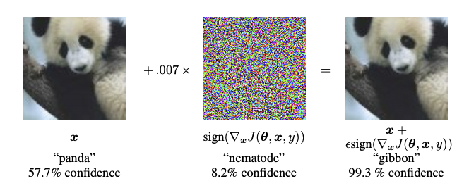
I hope this report provided you with an intuitive introduction to adversarial examples in deep learning. The techniques we discussed are inspired by the Fast Gradient Sign Method, as demonstrated by Goodfellow et al. in their paper - Explaining and Harnessing Adversarial Examples. Additionally, this paper discusses a wide variety of different adversarial attacks and, most notably, how to defend against them.
You might be wondering if adversarial examples are so negatively impactful why can’t we just train our networks to be adversarially robust. Well, of course, you can! This report could have been an overkill if I included it. This report is a part of a mini-crash course on adversarial examples and adversarial training in deep learning, so definitely stay tuned if you are interested to know more about this field, including training neural networks to be adversarially aware.
References
Add a comment

Iterate on AI agents and models faster. Try Weights & Biases today.