An Introduction to Adversarial Latent Autoencoders
In this article, we harness the latent power of autoencoders, one disentanglement at a time, and provide an example that you can try for yourself.
Created on June 13|Last edited on November 22
Comment
In the words of Yann LeCun, Generative Adversarial Networks (GANs) are "The most interesting idea in Machine Learning in the last 10 years". This is not surprising since GANs have been able to generate almost anything from high-resolution images of people "resembling" celebrities, building layouts and blueprints all the way to memes. Their strength lies in their incredible ability to model complex distributions.
While autoencoders have attempted to be as versatile as GANs, they have (at least until now) not had the same generative power as GANs and historically have learnt entangled representations. The authors of the paper draw inspiration from recent progress in GANs and propose a novel autoencoder which addresses these fundamental limitations. In the next few sections, we'll dive deeper and find out how.

Table of Contents
Preliminaries
Autoencoders
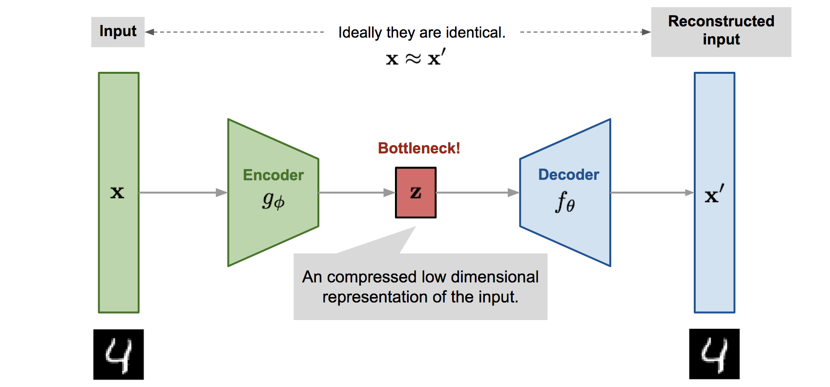
An autoencoder is a combination of an encoder function, , which takes in input data and converts it into a different representation; and a decoder function, , which takes this representation back to the original domain. Here is the latent representation of the input. Thus an encoder compresses high-dimensional input space (the data) into low dimensional latent space (the representation). While the decoder reconstructs the given representation back to the original domain. Thus, they can combine both generative and representational properties by learning an encoder-generator(decoder) map simultaneously.
GANs
A GAN stages a battle between two adversaries, namely, the Generator() and the Discriminator(). As the name suggests, a generator is responsible for learning the latent space(), which is a known prior , to generate new images, representing synthetic distribution , without directly encoding the image to that latent space as we were doing with an autoencoder. The discriminator, on the other hand, is responsible for telling apart the generated images from those present in the training dataset, which represents the true distribution . GANs aims at learning such that is as close as . This is achieved by playing a zero sum two player game with the discriminator. You can read more on autoencoder, GAN and latent representation here.

Adversarial Latent Autoencoders
Even though the autoencoders have been extensively studied, some issues have not been fully discussed and they are:
- Can autoencoders have the same generative power as GAN?
- Can autoencoders learn disentangled representations?
Points in the latent space holds relevant information about the input data distribution. If these points are less entangled amongst themselves, we would then have more control over the generated data, as each point contributes to one relevant feature in the data domain. The authors of Adversarial Latent Autoencoder held by Pidhorskyi et al., have designed an autoencoder which can address both the issues mentioned above jointly. Next, let's take a closer look at the architecture.
The official repo of the paper can be found here
Architecture
ALAE
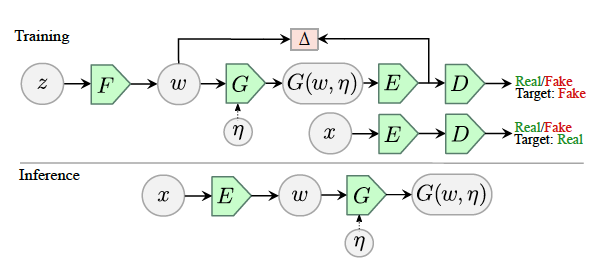
The ALAE architecture is a modification of the original GAN by decomposing the Generator and Discriminator networks into two networks such that: = and = . The architecture is shown in Figure 3. It's assumed that the latent space between both the decomposed networks is the same and is denoted as . Let's go through each network block one by one.
1. Mapping From Latent (F)
This network is responsible to convert the prior distribution to an intermediate latent () distribution, . It has been shown in this paper that an intermediate latent space, far imposed from the input space, tends to have better disentanglement properties. The authors of ALAE, have assumed to be a deterministic map in most general cases.
Thus takes in samples from known prior, , and outputs .
Network definition in Model class in model.py
## (F) Mapping from known prior p(z)->Wself.mapping_fl = MAPPINGS["MappingFromLatent"](num_layers=2 * layer_count,latent_size=latent_size,dlatent_size=latent_size,mapping_fmaps=latent_size,mapping_layers=mapping_layers)
In the generate method of the same class, this is how self.mapping_fl is used.
if z is None:z = torch.randn(count, self.latent_size)## (F) maps p(z) to latent distribution, Wstyles = self.mapping_fl(z)[:, 0]
2. Generator (G)
This is the good old generator from our GAN. But with two differences:
- The input to our old Generator is sampled directly from the latent space, whereas now the input to our generator is the intermediate latent space which you will soon realize is learned from the space of the input training data.
- The output of our old Generator is fed to the Discriminator which is nothing more than a binary classifier. In ALAE architecture design the output of is fed to an Encoder() as shown in the figure above.
The authors have assumed that might optionally depend on an independent noisy input, which is sampled from a known fixed distribution .
Thus the inputs to Generator() are and optionally . The output is given by,

where, is the conditional probability of generated image given and .
Network definition in Model class in model.py
## Generator (G) Takes in latent space and noiseself.decoder = GENERATORS[generator](startf=startf,layer_count=layer_count,maxf=maxf,latent_size=latent_size,channels=channels)
In the generator method, this is how self.decoder is used.
rec = self.decoder.forward(styles, lod, blend_factor, noise)
They must have named it adecoder because the Generator of GAN is similar to the Decoder of an autoencoder.
3. Encoder (E)
As the name suggests, Encoder(E) encodes the data space into latent space. The latent space between = and = is the same. That is, the Encoder should encode the data space to the same intermediate latent space, .
During training, the input to the Encoder is either real images from the true data distribution or generated images representing synthetic distribution . This is shown in figure 3.
The output of the Encoder when the input is drawn from the synthetic distribution is,

where, is the conditional probability distribution of the latent space given the data space, .
The output of the Encoder when the input is drawn from the true data distribution is,

Since ALAE is trained with an adversarial strategy, will eventually move towards . This also implies that move towards .
3.1 Matching the latent space
The assumption on the latent space implies that the output distribution of the the Encoder(), , is similar to the input distribution to the Generator (), .
This is achieved by minimizing the squared difference between both the distributions. Quite simple, yet quite wondrous.
In a vanilla autoencoder, the reconstruction loss such as the norm is calculated in the data space. This however does not reflect human visual perception. It has been observed that the computation of the norm in the image space is one of the reasons why autoencoders haven't been able to generate sharp images like GANs. This is where enforcing reciprocity in the latent space comes to the rescue.
The model definition in Model class is model.py.
## Encoder (E): Encodes image to latent space Wself.encoder = ENCODERS[encoder](startf=startf,layer_count=layer_count,maxf=maxf,latent_size=latent_size,channels=channels)
In the encoder method of the same class, this is how self.encoder is used.
## Encode generated images into ~WZ = self.encoder(x, lod, blend_factor)
In the forward method of the Model class, this is implemented this way.
## Known prior p(z)z = torch.randn(x.shape[0], self.latent_size)## generate method returns input(s) and output(rec) to generator.s, rec = self.generate(lod, blend_factor, z=z, mixing=False, noise=True, return_styles=True)## encode method returns encoder output(Z)Z, d_result_real = self.encode(rec, lod, blend_factor)## Mean squared error in the latent space-l2 norm.Lae = torch.mean(((Z - s.detach())**2))
4. Mapping To Latent (D)
This network takes is fed by the encoder and outputs a variable of shape (batch_size, 1) to be used as labels for binary classification by the discriminator.
During training it is used twice: once when the output of the encoder which is input for , is produced by the generator, and second when the output of the encoder is generated by real data as input.
Network definition in class Model in model.py.
self.mapping_tl = MAPPINGS["MappingToLatent"](latent_size=latent_size,dlatent_size=latent_size,mapping_fmaps=latent_size,mapping_layers=3)
In the forward method this is how self.mapping_tl is used.
## generator method returns the generated image.Xp = self.generate(lod, blend_factor, count=x.shape[0], noise=True)## encode method takes in real data x and return real labels._, d_result_real = self.encode(x, lod, blend_factor)## encode method takes in generated data and return fake label._, d_result_fake = self.encode(Xp.detach(), lod, blend_factor)
4. Mapping To Latent (D)
This network takes is fed by the encoder and outputs a variable of shape (batch_size, 1) to be used as labels for binary classification by the discriminator.
During training it is used twice: once when the output of the encoder which is input for , is produced by the generator, and second when the output of the encoder is generated by real data as input.
Network definition in class Model in model.py.
self.mapping_tl = MAPPINGS["MappingToLatent"](latent_size=latent_size,dlatent_size=latent_size,mapping_fmaps=latent_size,mapping_layers=3)
In the forward method, this is how self.mapping_tl is used.
## generator method returns the generated image.Xp = self.generate(lod, blend_factor, count=x.shape[0], noise=True)## encode method takes in real data x and return real labels._, d_result_real = self.encode(x, lod, blend_factor)## encode method takes in generated data and return fake label._, d_result_fake = self.encode(Xp.detach(), lod, blend_factor)
To summarize, the authors of ALAE have designed an Autoencoder(AE) architecture where:
- The latent distribution is learned by the input data to address entanglement.
- The output data distribution is learned by an adversarial strategy.
- To do both (1) and (2), autoencoder reciprocity is imposed in the latent space. This property relates to the ability of the architecture to reconstruct a data sample from its code and vice versa.
Style ALAE
Now that we have an understanding of the building blocks ALAE. Let's quickly go through the StyleALAE architecture which can generate 1024x1024 face images which is comparable to StyleGAN which is state of the art for face generation.
There are two components of StyleALAE:
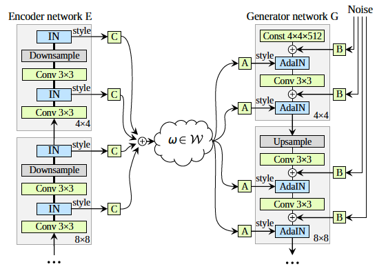
- The generator of ALAE is replaced with the generator of StyleGAN as shown in the right side of figure 4.
- The left side of figure 4 is a symmetrical Encoder so that style information can be extracted which drives the StyleGAN generator.
The style information is extracted from the layer by introducing Instance Normalization(IN) in that layer. This layer outputs channel-wise averages and standard deviation , which represent the style content in each layer. The IN layer provides normalization to the input in each layer. The style content of each such layer of the encoder is used as input by the Adaptive Instance Normalization (AdaIN) layer of the symmetric generator which is linearly related to the latent space . Thus, the style content of the encoder is mapped to the latent space via a multilinear map.
The authors have used progressive resizing during training. That is the training starts with a low-resolution image (4 x 4 pixels) and is gradually increased by blending in new blocks to Encoder and Generator.
Implementation
ALAE Training
The ALAE is a modification of a vanilla GAN architecture with some novel tweaks. Training of this architecture thus involves learning with respect to the Generator and Discriminator pair. A vanilla GAN is trained with a two step training procedure. By altering the training of the generator and the discriminator networks, the generator becomes more adept in fooling the discriminator, while the discriminator becomes better at catching the images artificially created by the generator. This forces the generator to come up with new ways to fool the discriminator and this cycle continues as such.
In case of the ALAE, given the assumption on the latent space, which ensures that the output distribution of the the Encoder(), , is similar to the input distribution to the Generator (), , a third training step is involved. These three updates as shown in the figure below.
- Step updates the discriminator, network blocks E and D.encoder_optimizer.zero_grad()loss_d = model(x, lod2batch.lod, blend_factor, d_train=True, ae=False)tracker.update(dict(loss_d=loss_d))loss_d.backward()encoder_optimizer.step()
- Step updates the generator, network blocks F and G.decoder_optimizer.zero_grad()loss_g = model(x, lod2batch.lod, blend_factor, d_train=False, ae=False)tracker.update(dict(loss_g=loss_g))loss_g.backward()decoder_optimizer.step()
- Step updates the latent space of the autoencoder, network blocks G and E.encoder_optimizer.zero_grad()decoder_optimizer.zero_grad()lae = model(x, lod2batch.lod, blend_factor, d_train=True, ae=True)tracker.update(dict(lae=lae))(lae).backward()encoder_optimizer.step()decoder_optimizer.step()

Experiments
Training the ALAE on MNIST
We tried to train the ALAE architecture on the MNIST dataset, however, ran into a bit of trouble. The authors have used their own library Dareblopy to prepare a training data generator. This library uses the TFRecord format. Unfortunately, we were not able to run the training script train_alae.py on colab.
After a lot of intensive debugging and fixes, we decided to implement the MLP based ALAE ourselves and train it on the MNIST dataset. The results you see are from our unofficial implementation and not from the official repo. You can check out our implementation in the link below:
Training a simple ALAE on MNIST
Note:
- Our implementation could not be checked for the correctness but it seems to be theoretically correct.
- It suffers from bad init and thus if your losses are not behaving as it should try to restart and run all. It worked out for us.
We trained the network for 75 epochs using the hyperparameters recommended by the authors. As described earlier, training ALAE involved three-stage of optimization. Thus we have three separate loss metrics to monitor the performance of the network. You can see the logged metrics below. 👇 Note that a smoothing factor of 0.5 is applied to show the trend properly.
- disc_loss: This loss is associated with the ability of the discriminator to predict fake(generated) images from the real ones. The discriminator loss reduces with lots of fluctuation which is common in adversary based training.
- gen_loss: This loss is associated with the ability of the generator to fool the discriminator. Our gen_loss seems to go up. But the generated images improved over time. It's not perfect but certainly, draw out the potential of our unofficial implementation.
- latent_loss: This loss determines the similarity of the latent space between F and G network and between E and D network. Thus unlike a GAN network where the latent space is simply sampled from a known distribution, this distribution is learned in ALAE. Over time the latent_loss reduces. We will soon see the effect of this.
The generated images after epoch 1, 25, 50, and 75 is shown below.
Run set
1
StyleALAE Experiments
The authors unleash their StyleALAE network on three datasets, FFHQ, LSUN, and Celeb-A. They train the network to generate, reconstruct and mix samples on these datasets. Let's take a look at their results.
Learning Style Representations
The authors train the StyleALAE described above on the FFHQ dataset which consists of 70k images of people's faces that are aligned and cropped at a resolution of . The dataset is split into 60k images for training and 10k images for testing. As expected, training a network on a large collection of high-resolution images needs significant computing resources. They use 8 x Titan RTX GPUs to train their network for 147 epochs of which 18 use training samples at the full resolution. They use the "progressive resizing" method where the input image resolution is first and grows progressively to the highest resolution over the course of training.
Interesting Tidbit Klaxon!!!!!
One of the interesting aspects here is that the StyleALAE is able to produce robust results at the highest resolution like the StyleGAN paper but spend only 1M in image training time at the highest resolution of while the StyleGAN spends 15M in image training time for the same resolution.
End of Interesting Tidbit Klaxon!!!!!
Quantitative Results
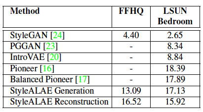
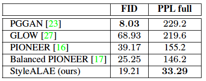
The FID or Fréchet Inception Distance is a measure of image visual quality and is generally accepted as an equivalent of human estimation of quality. The StyleALAE achieves very good FID scores but is still not as good as the StyleGAN per this metric. The table below shows the results on both the FFHQ and LSUN datasets.
What's interesting however is that while measuring the level of disentanglement of representations via the Perceptual Path Length (PPL) metric, the StyleALAE outperforms the StyleGAN as shown below:
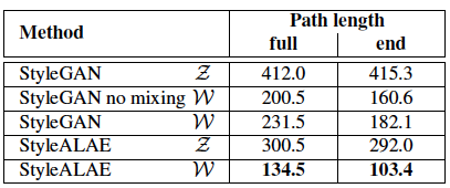
The next logical question to ask would be "How does the StyleALAE stack up against other comparable methods?". The answers to that question are also available courtesy of this ablation on the Celeb-A dataset:
Qualitative Results
We've re-run some of the generation, reconstruction, and mixing experiments the authors have shared in their repo and the results are below. Note that the pre-trained models for these experiments are available in the official repo. If you'd like to follow along, here's the colab notebook for your quick reference
Running Inference and Generating Results with Style ALAE
Generation
Here are some results of using the StyleALAE to generate some random images based on the three datasets it was trained on.
Run set
1
Summary
This is honestly one of the most impressive showings from an autoencoder architecture since sliced bread. It was a lot of fun for us to replicate some of the experiments and understand this work better. We hope this article has helped you in making this work more accessible, or on the very least has made you excited about interpolating between images. For any feedback feel free to drop us a note on Twitter: @DSaience, @ayushthakur0. Fin
Run set
1
Add a comment

Delia •
Sorry to disturb you, I encountered a problem running Colab named ‘ALAE Test’. I'm just a novice. I don't understand very well. Can you help me?
[INFO] After Epoch: 1 Loss: loss_d: 0.0790255, loss_g: 4.5910645, lae: 0.5456880
2020-12-10 01:37:06,946 logger INFO:
[1/60] - ptime: 202.42, loss_d: 0.0790255, loss_g: 4.5910645, lae: 0.5456880, blend: 1.000, lr: 0.001500000000, 0.001500000000, max mem: 2866.422852",
Traceback (most recent call last):
File "train_alae_new.py", line 329, in <module>
world_size=gpu_count)
File "/content/ALAE/launcher.py", line 131, in run
_run(0, world_size, fn, defaults, write_log, no_cuda, args)
File "/content/ALAE/launcher.py", line 96, in _run
fn(**matching_args)
File "train_alae_new.py", line 318, in train
save_sample(lod2batch, tracker, sample, samplez, x, logger, model_s, cfg, encoder_optimizer, decoder_optimizer)
File "train_alae_new.py", line 71, in save_sample
assert sample_in.shape[2] == needed_resolution
AssertionError
Reply

Sam Jackson •
Interesting post Ayush! Me and my friend were trying to reimplement this paper and were looking for resouces available on internet. Trust me this report is really helpful especially the fact that you have mapped the main components of the architectural design to the actual code in the official repo. Its a great help.
Finally we have an autoencoder that can be compared to GAN. I find autoencoders to be more interpretable and easy to implement.
1 reply

João Pedro Rodrigues Mattos •
Excelent post! There's a small mistake in the "architecture" section, though: the authors define G as G compose F, not as F compose G as it is stated in the post. The same occurs with D, which is defined in the original paper as D composes E and not the opposite! Congrats, once again, for the amazing post!
4 replies
Tags: Intermediate, Computer Vision, GenAI, Experiment, Research, GAN, Github, Panels, Plots, Slider, MNIST

Iterate on AI agents and models faster. Try Weights & Biases today.