How to train and evaluate an LLM router
This tutorial explores LLM routers, inspired by the RouteLLM paper, covering training, evaluation, and practical use cases for managing LLMs effectively.
Created on September 4|Last edited on September 12
Comment
Large language models have transformed business, showing impressive performance across various tasks, from natural language understanding to complex reasoning. However, deploying these models often requires balancing performance and cost. Advanced models like GPT-4o deliver high accuracy but at a high computational and financial cost. This creates a challenge in cost-sensitive applications where maintaining quality while managing expenses is crucial.
In this tutorial, we explore the concept of LLM routing, a strategy that helps navigate the trade-offs between performance and cost by intelligently directing queries to different models based on their complexity. We will cover what an LLM router is, why it’s needed, how it works, along with practical steps to train and evaluate one.
This project is heavily inspired by the recent paper RouteLLM: Learning to Route LLMs with Preference Data by Ong et al, so if you are interested in learning more, definitely check out the paper.

Table of contents
What is an LLM router?When do you need an LLM router?How does an LLM router work?Building and training an LLM routerCollecting training data Training an LLM routerEvaluating LLM routing performanceEvaluating cost/performance tradeoffsEvaluating response quality with Weave ConclusionRecommended readingAdditional resourses
What is an LLM router?
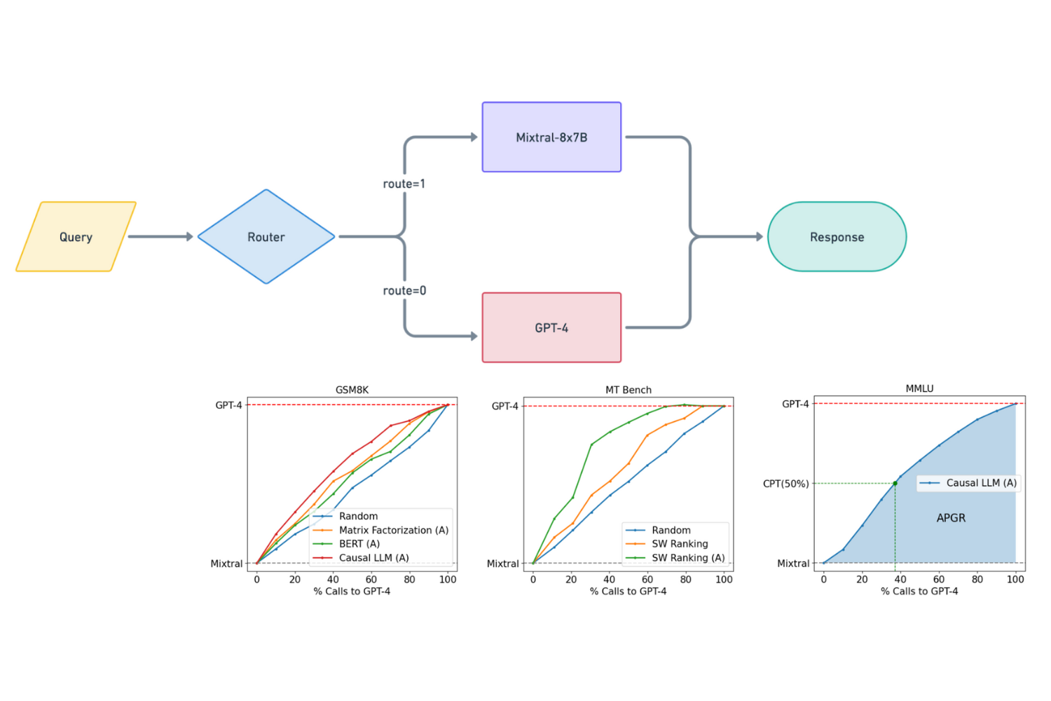
An LLM router is a system that dynamically directs queries to the most appropriate large language model based on the complexity of the task. It sends simpler queries to smaller, more cost-effective models, while reserving complex tasks for more powerful models, balancing performance and cost.
This approach optimizes resource allocation by balancing performance and cost, ensuring that computationally expensive models are used only when necessary. There are many different variations of LLM routers, but we will focus on building a router capable of routing between a "strong" and "weak" model. Examples of strong models are GPT-4o and Claude 3.5 Sonnet, whereas a weak model might be Mixtral-8x7B or GPT-4o Mini.

Diagram of an LLM Router [1]
When do you need an LLM router?
You need an LLM router when deploying LLMs in applications where there is a need to balance performance quality with cost constraints. This is particularly important in scenarios where queries vary widely in complexity, such as in chatbots, customer service systems, and other interactive AI solutions.
If all queries are sent to a high-performing model like GPT-4o, the costs can quickly become prohibitive. An LLM router is useful when you want to maintain high-quality responses without incurring the full expense of using a strong model for every interaction. By routing queries to the most appropriate model, the system reduces costs while maintaining an acceptable level of performance, making it ideal for cost-sensitive applications that still require accurate and timely responses.
How does an LLM router work?
An LLM router works by learning which types of queries are more likely to produce favorable results when handled by weaker models. During training, the router is exposed to examples of queries and their corresponding performance outcomes when routed to either the strong or weak model. By analyzing these patterns, the router learns to identify characteristics of queries that typically require the stronger model to achieve high-quality results.
When a new query arrives, the router uses this learned knowledge to predict the likelihood of each model’s success. If the query resembles those that previously led to better results with the strong model, the router directs it there. Conversely, if the query is likely to be adequately handled by the weaker model, it is routed accordingly. This dynamic decision-making process optimizes performance while controlling costs, ensuring that each query is handled by the model best suited to deliver favorable results based on past learnings.
Building and training an LLM router
To build and train an LLM router, the primary goal is to develop a model that can decide whether to route a query to a strong or weak model based on the likelihood of achieving the desired performance. This involves collecting or creating a labeled dataset, training a classifier to predict the best routing decision, and fine-tuning the model to optimize performance.
Collecting training data
To train an LLM router, we'll use a dataset generated through a systematic process designed to capture the performance differences between strong and weak models across a wide range of queries. This dataset serves as the foundation for teaching the router which queries are best handled by each model.
The dataset, available on HuggingFace at this link, was generated using queries and responses initially sourced from the Nectar dataset. Responses from GPT-4 were selected directly from this dataset. Following this, responses from the weaker model, Mixtral-8x7B, were generated for the same queries. GPT-4 was then used as an automated judge to generate scores ranging from 1 to 5, reflecting how well the Mixtral responses matched the GPT-4 responses. These scores provide a measure of alignment between the outputs of the two models.
For example, if a response receives a rating of 4 or higher, it is considered sufficiently good for the weak model, while ratings below this threshold suggest that the strong model should handle the query. This labeled dataset thus enables the LLM router to learn and make informed routing decisions, guiding it to allocate queries to the most appropriate model based on historical performance outcomes.
For your use case, it will most likely make sense to use domain specific data relevant to your use-case. Luckily, Weave by Weights & Biases provides a great solution for anyone looking to manage LLM data generated in production.
For example, let's say you have a inference pipeline which uses GPT-4o, and you would like to log your examples. Simply add the @weave.op decorator, which will log all inputs and outputs to your model.
import weaveweave.init("project_name")@weave.opdef run_inference(prompt):return gpt4o_inference(prompt)
We're able to log responses from GPT-4o by using the @weave.op decorator, which will log the inputs and outputs to our run_inference function. Later, we can download this data from Weave, and generate responses from other models, such as Mixtral-8x7B, and then use GPT-4o to compare both outputs, which will result in a dataset which could be used to train a LLM router. This can ultimately result in cost savings, while only sacrificing marginal performance.
Additionally, Weave provides tools to add feedback to examples, so that you can later use this feedback to further improve your models. Using Weave's Python SDK, you can log every inference call made by your models, capturing not just the raw input and output but also user feedback associated with each interaction. This feedback data can be used as additional supervision for training new models.
Here's an example of how you could add feedback to a model output, using Weave:
import weaveweave.init("project_name")@weave.opdef run_inference(prompt):return gpt4o_inference(prompt)# Execute the inference and get the result and call objectresult, call = run_inference.call("example input")# Add feedback with a value between 1 and 5feedback_value = 4 # Example value between 1 and 5call.feedback.add("rating", {"value": feedback_value})
Ultimately, integrating feedback loops like these into your model evaluation process with Weave empowers your team to rapidly iterate on existing data pipelines, ensuring your future models can take full advantage of past production data.
Training an LLM router
Now we will focus on developing a routing system for large language models by training a classifier to decide whether a query should be handled by a strong model, such as GPT-4o, or a weaker, cost-effective model like Mixtral-8x7B. To optimize routing decisions, we utilize a dataset containing GPT-4o and Mixtral responses, rated on a scale of 1 to 5 based on how well Mixtral's answers align with those of the GPT-4o response.
It may sound a bit strange that we are using GPT-4o to rate the quality of responses generated by GPT-4o and Mixtral (GPT-4o comparing it's own answers to another model). However, since we are asking the model to compare how well the Mixtral responses match the GPT-4o responses, I believe there is less risk that the model will be biased towards its own responses, as it's simply comparing how well the Mixtral responses match up to the GPT-4o responses.
Responses rated 4 or higher are considered sufficient for the weaker model, while those rated below 4 indicate a need for the stronger model. This code trains a binary classifier that learns these routing patterns. Using Torch and the Sentence Transformers library, the model is trained to predict whether a query should be routed to the weaker or stronger model based on its alignment score, aiming to minimize cost without sacrificing performance.
import torchimport osfrom torch import nnfrom torch.utils.data import Dataset, DataLoader, WeightedRandomSamplerfrom sentence_transformers import SentenceTransformerfrom sklearn.model_selection import train_test_splitfrom datasets import load_datasetimport wandb # Import W&B# Initialize W&Bwandb.init(project="router") # Set your project name# Load the dataset from Hugging Facedataset = load_dataset("routellm/gpt4_dataset")# Convert the training data to pandas DataFrame for easier manipulationtrain_df = dataset["train"].to_pandas()# Define the scoring threshold for routing labelstrain_df["routing_label"] = train_df["mixtral_score"].apply(lambda x: 0 if x >= 4 else 1) # Binary classification labels# Extract prompts and labels for trainingsentences = train_df["prompt"].tolist()labels = train_df["routing_label"].tolist()# Split the data into training and validation setssentences_train, sentences_val, labels_train, labels_val = train_test_split(sentences, labels, test_size=0.2, random_state=42)# Create a custom PyTorch datasetclass TrainingDataset(Dataset):def __init__(self, sentences, labels):self.sentences = sentencesself.labels = labelsdef __len__(self):return len(self.sentences)def __getitem__(self, idx):sentence = self.sentences[idx]label = self.labels[idx]return sentence, torch.tensor(label, dtype=torch.float) # Use float for BCEWithLogitsLoss# Create DataLoaderstrain_data = TrainingDataset(sentences_train, labels_train)val_data = TrainingDataset(sentences_val, labels_val)train_loader = DataLoader(train_data, batch_size=32)val_loader = DataLoader(val_data, batch_size=32, shuffle=True) # Validation loader remains unchanged# Define the classifier model with trainable transformer backboneclass Classifier(nn.Module):def __init__(self, transformer_model_name):super(Classifier, self).__init__()self.transformer = SentenceTransformer(transformer_model_name)self.fc1 = nn.Linear(self.transformer.get_sentence_embedding_dimension(), 512)self.fc2 = nn.Linear(512, 256)self.fc3 = nn.Linear(256, 1) # Single output neuron for binary classificationself.relu = nn.ReLU()def forward(self, sentences):embeddings = self.transformer.encode(sentences, convert_to_tensor=True) # Generate embeddings in the forward passx = self.relu(self.fc1(embeddings))x = self.relu(self.fc2(x))logits = self.fc3(x) # Output single logit for binary classificationreturn logits# Initialize the classifiermodel = Classifier(transformer_model_name='sentence-transformers/all-distilroberta-v1')# Use GPU if it's availabledevice = torch.device("cuda" if torch.cuda.is_available() else "cpu")model = model.to(device)# Define loss function and optimizercriterion = nn.BCEWithLogitsLoss() # Use BCEWithLogitsLoss for binary classification with one output neuronoptimizer = torch.optim.Adam(model.parameters(), lr=0.001)# Number of epochsn_epochs = 10# Directory to save the best modelruns_dir = "runs"os.makedirs(runs_dir, exist_ok=True)# Initialize best validation loss with infinitybest_valid_loss = float('inf')# Log hyperparameters to W&Bwandb.config = {"learning_rate": 0.001,"epochs": n_epochs,"batch_size": 32,}def validate(model, val_loader, criterion, device):"""Perform validation and return the loss, accuracy, and percentage of predictions for each class."""model.eval()valid_loss = 0.0valid_correct = 0total_predictions = []with torch.no_grad():for sentences, labels in val_loader:sentences = list(sentences)labels = labels.to(device)# Forward passoutputs = model(sentences).squeeze(1)# Compute lossloss = criterion(outputs, labels)valid_loss += loss.item()predictions = torch.round(torch.sigmoid(outputs))valid_correct += (predictions == labels).sum().item()total_predictions.extend(predictions.cpu().numpy())valid_loss /= len(val_loader)valid_accuracy = valid_correct / len(val_loader.dataset)return valid_loss, valid_accuracy# Initial validation of the untrained modelinitial_valid_loss, initial_valid_accuracy = validate(model, val_loader, criterion, device)print(f'Initial Validation Loss: {initial_valid_loss:.4f}, Initial Validation Accuracy: {initial_valid_accuracy:.4f}')wandb.log({"epoch": 0,"valid_loss": initial_valid_loss,"valid_accuracy": initial_valid_accuracy,})for epoch in range(n_epochs):# Trainingmodel.train()train_loss = 0.0train_correct = 0for sentences, labels in train_loader:sentences = list(sentences) # Convert tensor of strings back to list for transformerlabels = labels.to(device)# Clear the gradientsoptimizer.zero_grad()# Forward passoutputs = model(sentences).squeeze(1) # Squeeze output to match shape [batch_size]# Compute lossloss = criterion(outputs, labels)# Backward pass and optimizationloss.backward()optimizer.step()train_loss += loss.item()predictions = torch.round(torch.sigmoid(outputs)) # Convert logits to probabilities and then round to 0 or 1train_correct += (predictions == labels).sum().item()train_loss /= len(train_loader)train_accuracy = train_correct / len(train_loader.dataset)# Validation after each epochvalid_loss, valid_accuracy = validate(model, val_loader, criterion, device)# Log metrics to W&Bwandb.log({"epoch": epoch + 1,"train_loss": train_loss,"train_accuracy": train_accuracy,"valid_loss": valid_loss,"valid_accuracy": valid_accuracy,})print(f'Epoch {epoch+1}/{n_epochs}, Training Loss: {train_loss:.4f}, Training Accuracy: {train_accuracy:.4f}, Validation Loss: {valid_loss:.4f}, Validation Accuracy: {valid_accuracy:.4f}')# Save the model if it's the best so farif valid_loss < best_valid_loss:best_valid_loss = valid_losstorch.save(model.state_dict(), os.path.join(runs_dir, 'best_model.pt'))print('Training complete.')wandb.finish() # Finish the W&B run
Fine-tuning the LLM router involves training a classifier that determines whether a query should be routed to a strong or weak model based on its complexity. The training process starts by loading a labeled dataset from HuggingFace, which contains queries and their performance scores from both strong and weak models. This dataset is converted into a pandas DataFrame to simplify manipulation. Labels are created based on a performance threshold: queries that score high enough with the weak model (e.g., a score of 4 or above) are labeled as suitable for that model, while lower scores indicate the need for the strong model.
The data is then split into training and validation sets using train_test_split, which ensures that the model is trained on one portion of the data and validated on another, allowing for the evaluation of its performance on unseen data. To handle the data efficiently, a custom PyTorch Dataset class is defined, structuring the queries and their labels into batches that can be shuffled and processed during training using the DataLoader utility.
The classifier model is constructed with a trainable transformer backbone from the Sentence Transformers library, which generates embeddings for the input sentences. These embeddings are passed through a series of fully connected layers with ReLU activations, culminating in a single output neuron that provides the logit for binary classification. The loss function used is BCEWithLogitsLoss, which is well-suited for binary classification tasks like routing decisions.
During each epoch, the model is trained on the training set to minimize the classification loss and improve accuracy. After training, the model's performance is evaluated on the validation set, allowing for the monitoring of its generalization to new data. Performance metrics such as training and validation loss and accuracy are logged throughout the process using Weights & Biases, enabling real-time tracking and analysis of the model’s progress.
As the model trains, it saves its state whenever it achieves a lower validation loss compared to previous iterations. This checkpointing ensures that the best version of the model is preserved, helping to avoid using models that have overfit the training data. The training concludes when all epochs are completed, and the Weights & Biases' run is finalized, consolidating the results of the experiment. The trained model is then ready to be deployed within the LLM routing system, where it will use its learned knowledge to dynamically decide the optimal model for each query, balancing performance with cost considerations.
Here are the training logs for my router:
Run: good-forest-15
1
Evaluating LLM routing performance
We use two key metrics—Performance Gap Recovered (PGR) and Call-Performance Threshold (CPT)—to evaluate routing effectiveness. PGR measures how much of the performance gap between a strong and a weak model the routing system can recover. For instance, if GPT-4o achieves 100% accuracy and Mixtral-8x7B achieves 86%, a routing model that reaches 93% has recovered half of the gap. This system allows tuning the routing model by adjusting thresholds that define when to route to the strong model based on query complexity and confidence levels.
CPT, on the other hand, quantifies the minimum percentage of queries that must be routed to the strong model to achieve a desired PGR level. For example, CPT(50%) indicates that half of the performance gap can be recovered with a certain percentage of calls to the strong model. Lower CPT values suggest a more efficient routing model that maintains high performance with fewer calls to the more expensive model. The performance/cost trade-off chart illustrates this balance, showing how accuracy responds to varying degrees of reliance on the strong model. Decision-makers can use this chart to identify optimal cost-saving strategies without sacrificing too much performance.
Here's an example of what a performance/cost trade-off chart looks like:

Evaluating cost/performance tradeoffs
To evaluate the routing strategy, CPT values are calculated to measure how efficiently the routing model balances performance and cost. By targeting specific PGR levels, the system identifies the minimal reliance on the strong model needed to achieve desired accuracy. A detailed analysis with 1000 evaluation "bins" helps determine the percentage of calls to the strong model required to reach PGR targets, such as 50% or 80%. This approach allows for precise identification of the optimal balance between performance recovery and cost, demonstrating the routing model’s effectiveness in dynamic query allocation.
In this context, bins refer to divisions of the evaluation dataset that represent different levels of reliance on the strong model (e.g., GPT-4o) during the routing process. Each bin corresponds to a specific percentage of queries that are routed to the strong model, allowing us to systematically evaluate how performance changes as more or fewer queries are sent to it.
For example, if we use 1000 bins, the first bin would represent routing 0.1% of the queries to the strong model, the second bin 0.2%, and so on, up to 100%. By sorting the model's confidence scores (logits) and progressively increasing the percentage of queries directed to the strong model, we create a series of bins that capture different routing scenarios.
Evaluating accuracy across these bins helps to visualize the trade-off between performance and cost, showing how much of the performance gap can be recovered at each level of strong model usage. This approach is crucial for calculating CPT values, as it pinpoints the minimum percentage of calls required to achieve specific performance targets.
Here’s some code that calculates CPT(50%) and CPT(80%) scores, along with the performance/cost trade-off chart for showing how performance improves as more calls to strong model are made.
import torchimport matplotlib.pyplot as pltfrom torch import nnfrom sentence_transformers import SentenceTransformerfrom datasets import load_datasetimport wandb# Initialize WandB projectwandb.init(project="router_eval", name="CPT_Evaluation")# Define the trained model class and load the modelclass Classifier(nn.Module):def __init__(self, transformer_model_name):super(Classifier, self).__init__()self.transformer = SentenceTransformer(transformer_model_name)self.fc1 = nn.Linear(self.transformer.get_sentence_embedding_dimension(), 512)self.fc2 = nn.Linear(512, 256)self.fc3 = nn.Linear(256, 1)self.relu = nn.ReLU()def forward(self, sentences):embeddings = self.transformer.encode(sentences, convert_to_tensor=True)x = self.relu(self.fc1(embeddings))x = self.relu(self.fc2(x))return self.fc3(x)model = Classifier('sentence-transformers/all-distilroberta-v1')model.load_state_dict(torch.load('runs/best_model.pt'))device = torch.device("cuda" if torch.cuda.is_available() else "cpu")model.to(device).eval()# Load evaluation datadataset = load_dataset("routellm/gpt4_dataset")eval_df = dataset["validation"].to_pandas()sentences_eval = eval_df["prompt"].tolist()labels_eval = eval_df["mixtral_score"].tolist()def calculate_accuracy(predictions, labels):correct = 0for pred, label in zip(predictions, labels):if pred == 1: # Routed to the strong modelcorrect += 1 # Always considered correctelif pred == 0 and label >= 4: # Routed to the weak model and label indicates correctcorrect += 1 # Correct if the label meets the thresholdreturn correct / len(predictions) if predictions else 0# Generate logits using the modeldef generate_logits(model, sentences, labels):logit_buffer = []for sentence, label in zip(sentences, labels):with torch.no_grad():output = model([sentence]).squeeze(1)prob_strong = torch.sigmoid(output).item()logit_buffer.append((prob_strong, 1 - prob_strong, label))return logit_buffer# Evaluate the model across binsdef evaluate_model_across_bins(logit_buffer, num_bins):bin_accuracies = []for pct in range(1, num_bins + 1):max_calls = int((pct / num_bins) * len(logit_buffer))sorted_buffer = sorted(logit_buffer, key=lambda x: x[0], reverse=True)predictions = [1 if i < max_calls else 0 for i in range(len(sorted_buffer))]true_labels = [lbl for _, _, lbl in sorted_buffer]accuracy = calculate_accuracy(predictions, true_labels)bin_accuracies.append((pct * 100 / num_bins, accuracy))return bin_accuracies# Plot and log accuracies with matplotlib for 1000-bin chartsdef plot_and_log_accuracies(bin_accuracies, title, log_name, target_accuracy=None, cpt=None):percentages, accuracies, cpt_values = zip(*bin_accuracies)plt.figure()plt.plot(percentages, accuracies, marker='o')plt.xlabel('% Calls to Strong Model')plt.ylabel('Accuracy')plt.title(title)plt.grid(True)# Add dashed lines for target accuracy and CPT, if providedif target_accuracy is not None:plt.axhline(y=target_accuracy, color='r', linestyle='--', label='Target Accuracy')if cpt is not None:plt.axvline(x=cpt, color='g', linestyle='--', label=f'CPT Value ({cpt:.2f})')# Annotate the actual CPT valueplt.text(cpt, target_accuracy, f'{cpt:.4f}', color='g', fontsize=9, ha='right', va='bottom')plt.legend()plt.savefig(f"{log_name}.png")wandb.log({log_name: wandb.Image(f"{log_name}.png")})plt.close()logit_buffer = generate_logits(model, sentences_eval, labels_eval)bin_accuracies_1000 = evaluate_model_across_bins(logit_buffer, 1000)# Find weak and strong model accuraciesweak_accuracy = calculate_accuracy([0] * len(labels_eval), labels_eval)strong_accuracy = calculate_accuracy([1] * len(labels_eval), labels_eval)# Calculate CPT values for 50% and 80% PGRtarget_accuracy_50 = (strong_accuracy - weak_accuracy) * 0.5 + weak_accuracytarget_accuracy_80 = (strong_accuracy - weak_accuracy) * 0.8 + weak_accuracycpt_50 = min(bin_accuracies_1000, key=lambda x: abs(x[1] - target_accuracy_50))[0]cpt_80 = min(bin_accuracies_1000, key=lambda x: abs(x[1] - target_accuracy_80))[0]# Log CPT valueswandb.log({"CPT_50": cpt_50, "CPT_80": cpt_80})# Plot and log the 1000-bin accuracy chartsplot_and_log_accuracies(bin_accuracies_1000, 'CPT 50 Evaluation (1000 Bins)', 'CPT 50 Chart', target_accuracy_50, cpt_50)plot_and_log_accuracies(bin_accuracies_1000, 'CPT 80 Evaluation (1000 Bins)', 'CPT 80 Chart', target_accuracy_80, cpt_80)wandb.finish()
CPT values are calculated to determine the minimum percentage of queries that must be routed to the strong model to achieve a specific level of performance improvement, known as Performance Gap Recovered (PGR). The process involves generating logits (predictions) from the trained routing model for each query, which indicate the confidence of the model in routing the query to the strong model.
These logits are sorted in reverse by confidence, and the model's accuracy is evaluated across multiple bins, each representing an increasing percentage of queries routed to the strong model. 1000 bins are used to assess how accuracy scales as more queries are directed towards the strong model, ranging from 0% to 100%, at discrete intervals of .1%.
Target accuracies are then set based on the desired PGR levels (e.g., 50% or 80%). The CPT value is identified as the point on the accuracy curve where the performance first meets or exceeds the target accuracy. This value represents the minimum fraction of queries that must be handled by the strong model to achieve the specified PGR, helping to balance performance and cost effectively. Additionally, we identify confidence thresholds (alpha) which will results in around 50% and 80% of calls using the strong model. This effectively allows us to tune our router to be more or less likely to route to the strong model, depending on our cost constraints.
Here are the performance/cost trade-off charts for my router:
Run: CPT_Evaluation
1
The charts show performance/cost trade-off's for the CPT(50%) and CPT(80%) evaluations. The CPT(80%) chart demonstrates that nearly 49.3% of calls to the strong model are required to meet the target accuracy of achieving 80% of the performance gap recovery between the strong and weak models. The CPT(50%) chart shows that about 22.8% of calls to the strong model are needed to reach the 50% performance gap recovery target. These results show the trade-off between using the strong model and achieving desired performance levels, showing that significant performance gains can be realized without routing all queries to the strong model.
Evaluating response quality with Weave
To gain deeper insights into how our model responds when using the router, we utilize Weave evaluations on our dataset. Weave is a powerful tool for streamlining evaluations, offering a quick and intuitive way to visualize how models respond to various queries.
While performance metrics are often the main focus, Weave goes further by logging individual responses directly to an interactive dashboard. This setup allows for easy comparison of responses side-by-side, making it simple to identify how different models handle the same query. This detailed examination of specific responses not only highlights the strengths and weaknesses of each model but also provides a clear view of where improvements can be made, giving machine learning practitioners the information needed to refine their models effectively.
Here's some code that evaluates our router with Weave!
import torchimport torch.nn as nnfrom sentence_transformers import SentenceTransformerimport pandas as pdimport weavefrom weave import Evaluationimport asynciofrom datasets import load_datasetfrom weave import Dataset# Define the classifier model with a trainable transformer backboneclass Classifier(nn.Module):def __init__(self, transformer_model_name):super(Classifier, self).__init__()self.transformer = SentenceTransformer(transformer_model_name)self.transformer.train()self.fc1 = nn.Linear(self.transformer.get_sentence_embedding_dimension(), 512)self.fc2 = nn.Linear(512, 256)self.fc3 = nn.Linear(256, 1) # Single output neuron for binary classificationself.relu = nn.ReLU()def forward(self, sentences):embeddings = self.transformer.encode(sentences, convert_to_tensor=True) # Generate embeddingsx = self.relu(self.fc1(embeddings))x = self.relu(self.fc2(x))logits = self.fc3(x) # Output single logit for binary classificationreturn logits# Sample alpha threshold for routingalpha = 0.23591 # Adjust this value based on your routing needs# Initialize the classifier model with the desired transformertransformer_model_name = 'sentence-transformers/all-distilroberta-v1'model = Classifier(transformer_model_name=transformer_model_name)model.load_state_dict(torch.load('runs/best_model.pt'))device = torch.device("cuda" if torch.cuda.is_available() else "cpu")model = model.to(device)# Load dataset from Hugging Face and convert to pandas dataframedataset = load_dataset("routellm/gpt4_dataset")val_df = dataset["validation"].to_pandas()# Initialize Weaveweave.init('router-example')# Define a scoring function that checks if the chosen response matches the expected one@weave.op()def match_score(expected: str, model_output: dict) -> dict:# Check if the chosen response matches the expected responsereturn {'match': expected == model_output['generated_text']}# Create evaluation examples directly from the dataframe for speedexamples = [{"prompt": row['prompt'],"expected": row['mixtral_response'] if row['mixtral_score'] >= 4 else row['gpt4_response'],"gpt4_response": row['gpt4_response'],"mixtral_response": row['mixtral_response'],}for _, row in val_df.head(100).iterrows() # just evaluate 100 samples]# Create a Dataset object with examplesdataset_obj = Dataset(name='gpt4_dataset_example', rows=examples)@weave.op()def run_inference(prompt: str, gpt4_response: str, mixtral_response: str) -> dict:model.eval()with torch.no_grad():# Forward pass through classifier to get routing scorelogits = model([prompt]).squeeze()score = torch.sigmoid(logits).item() # Convert logit to probability score between 0 and 1# Decision logic based on score and alphachosen_response = gpt4_response if score > alpha else mixtral_response# Return the chosen responsereturn {'generated_text': chosen_response,}# Create an evaluation object with examples and the scoring functionevaluation = Evaluation(dataset=dataset_obj, scorers=[match_score])# Run the evaluation asynchronously on the functionasyncio.run(evaluation.evaluate(run_inference))print('Evaluation complete.')
This code sets up an evaluation system for an LLM router using Weave, which involves building a classifier model, loading data, and running an evaluation on the responses generated by the router. The classifier model is initialized with a Sentence Transformer backbone, which generates embeddings for input sentences. These embeddings are passed through fully connected layers to produce a single logit for binary classification, used to determine if the query should be routed to a strong model like GPT-4o or a weaker model like Mixtral.
The evaluation data is loaded from HuggingFace and converted into a pandas DataFrame, where each prompt is linked with responses from GPT-4o and Mixtral. A decision function evaluates whether the response matches the expected outcome based on a threshold (alpha), which defines if the strong model should be used. The responses are then logged into Weave’s system for comparison.
A key details when using Weave is that large datasets, such as those used for evaluation, must be converted into a Dataset object. This conversion is important because Weave requires dataset objects when using large datasets during the evaluation process. Similarly, any large object that is accessed in the inference function, must also be structured as a dataset object.
In this evaluation, we do not use the models to generate new responses since the responses from GPT-4o and Mixtral are already stored in the dataset. This evaluation is primarily intended to provide a better visualization of how the models respond to various queries, enabling a detailed comparison of their outputs. The alpha value used in the routing decision was previously obtained when calculating our CPT(50%) and CPT(80%) scores, guiding the evaluation process by determining the confidence threshold for routing decisions. This setup allows us to focus on examining the model's decision-making and its impact on response quality, rather than generating new data during the evaluation.
After running this evaluation, you can easily visualize the responses chosen for each query! Here's a screenshot inside Weave of what my results look like:

Conclusion
This project illustrates how LLM routing can effectively balance performance and cost in deploying large language models. By strategically routing queries based on complexity, the system maintains high response quality while reducing reliance on expensive models.
Key metrics like PGR and CPT help evaluate and fine-tune the routing strategy, showcasing the potential for significant cost savings without sacrificing performance. This approach facilitates scalable, cost-effective AI deployments, broadening access to advanced capabilities across various applications.
Additionally, the usage of Weave provides a quick and easy way to visualize model performance.
Recommended reading
Building a real-time answer engine with Llama 3.1 405B and W&B Weave
Infusing llama 3.1 405B with internet search capabilities!!
Building the worlds fastest chatbot with the Cerebras Cloud API and W&B Weave
A guide to getting started using the Cerebras Cloud API with W&B Weave.
YOLOv9 object detection tutorial
How to use one of the worlds fastest and most accurate object detectors to run inference, display on your webcam using OpenCV and tracking your results.
How to fine-tune Phi-3 Vision on a custom dataset
Here's how to fine tune a state of the art multimodal LLM on a custom dataset
Additional resourses
Building an LLM Router for High-Quality and Cost-Effective Responses
This blog post provides a comprehensive guide to building one of our most robust router models (causal LLM) at Anyscale.

RouteLLM: Learning to Route LLMs with Preference Data
The "RouteLLM" paper presents a method for optimizing LLM deployment by routing queries between models to balance cost and performance.
Add a comment
Iterate on AI agents and models faster. Try Weights & Biases today.