GANspace: An Overview of Generative Adversarial Networks
This article provides an overview of the unsupervised discovery of interpretable feature directions in pre-trained generative adversarial networks (GANs).
Created on December 31|Last edited on December 5
Comment
Since its inception in 2014, Generative Adversarial Networks (aka GANs) has been at the forefront of Generative Modeling research. GANs, with their millions of parameters, have found extensive usage in modeling probability densities of various complex data formats and generating ultra-realistic samples. These include photorealistic images, near-human speech synthesis, music generation, photorealistic video synthesis, etc.
These, along with its likelihood-free density estimation framework, GANs have found application in various challenging problems. One such area of interest involves modeling densities with interpretable conditionals, to generate samples having certain desired features. For example, controlling the intensity of certain features of images of human faces like — smile, color, orientation, gender, facial structure, etc.
Among the various inherent problems in training GANs, this problem poses an additional challenge, i.e., lack of proper metric for atomically labeling intensities of sample features, which hinders the trivial solution of training the GAN under the supervision of the conditional. In simpler terms, it is virtually impossible to have a dataset with a measure for the number of smiles in a headshot, thus making it impossible to perform the training in a supervised setting.
This work studies a novel approach for discovering GAN controls in the Gaussian prior, in an unsupervised way. More importantly, this method doesn't need any retraining of GANs. This makes it convenient to generate controlled samples from pretrained state-of-the-art GAN architectures, like BigGAN, StyleGAN, StyleGAN2, etc.
Table of Contents
Table of ContentsBrief Primer on Relevant BackgroundGenerative Adversarial NetworksSpectral DecompositionImportant TakeawayPrior Space Exploration in GANsFinding Principal DirectionsBigGAN Based Architectures (Isotropic Priors)Interpreting Principal Feature Directions
Brief Primer on Relevant Background
Generative Adversarial Networks
It is not a surprise that real-world data arises from a remarkably complex probability distribution. This complicated nature renders any likelihood-based density estimator useless. More formally, the likelihood integral of the Bayesian framework for posterior estimation becomes intractable to evaluate.
One trivial solution for this problem is to avoid the exact evaluation of the integral and approximate it using a simpler distribution, , called a variational lower bound. For example, VAEs by Kingma et. al. uses as the variational lower bound. However, this approximation doesn't capture the intricacies of the likelihood distribution properly resulting in poor quality samples.
GANs, with its novel game-theoretic framework, solves this problem by avoiding the likelihood evaluation step by introducing a neural network between the prior and the posterior. First proposed by Goodfellow et.al. in his seminal paper "Generative Adversarial Networks", GANs model the density estimation process as a zero-sum game between two competing players. One of the players, the generator G, is modelled as a parametric function between the prior (commonly isotropic gaussian ) and posterior space . The discriminator D, parameterized by , tries to classify the samples between real and synthetic. For each optimization step, a player takes turns to improve its result, until a Nash equilibrium is attained. The formal objective is defined as follows.
Spectral Decomposition
Among the various canonical forms of matrix representation, the eigenvector-eigenvalue form finds the most usage in machine learning literature. This is evident by its prevalence in recommendation systems literature, especially in dimensionality reduction. Eigenvalues have also found extensive usage in invertible neural networks, where singular values of weight matrices play a crucial role in preserving the isometry of layers.
Formal Definition
Given a square matrix considered as a linear map from some vector space onto itself, i.e. , the eigenvector of the vector space, is defined as the vector whose linear transformation using , results only in a scale transformation by some constant . i.e., , where is the known as the eigenvalue.
For a set of all eigenvectors and eigenvalues,
, where is the rank of the matrix , is the matrix of eigenvectors whose column denotes the eigenvector on , is a diagonal matrix, where each entry is the eigenvalue of the corresponding eigenvector.
Therefore, is defined as the eigen decomposition of matrix .
Despite the intuitive nature and widespread popularity of eigendecomposition, in practice, a generalized version of eigendecomposition, called singular value decomposition (SVD) is used. SVD removes the square matrix limitation of the eigendecomposition, by considering two vector spaces, row space() and column space (), instead of one. The final decomposition provides orthonormal basis vectors(analogous to eigenvectors) of the row space and column space, and the singular values(analogous to eigenvalues) accompanying it. This orthonormality allows accurate calculation of matrix inverses, making the decomposition computationally efficient.
Formal Definition
Let be a linear map from a vector space to a vector space , i.e., . Let be the matrix of singular vectors in , and be the matrix of singular vectors in . Without loss of generality from the previous defintion, , where is a diagonal matrix of singular values. Thus the singular value decomposition is defined as Since is an orthogonal matrix, hence, the final decomposition is defined as:
Important Takeaway
The methods discussed above decomposes a matrix in linearly independent vectors. Hence, for a full-rank matrix decomposition, the eigenvectors/singular vectors form a basis on the vector space(s). One important observation is that, since the vectors are normalized and form a basis, they can be used to represent any vector in the space, by performing an arbitrary linear combination of the vectors.
Note: The top-k column space singular vectors, (i.e., column space singular vectors associated with the largest singular values), are called the k-principal components. The process representing a matrix decomposition, by selecting dominant singular vectors is also known as Principal Component Analysis (PCA).
Prior Space Exploration in GANs
Interpretable GAN control discovery, aka, latent space disentanglement in GANs, has been a heavily studied problem. The most notable work by Chen et. al., called InfoGAN, used mutual information between the posterior and a conditional vector passed along with prior.
However, this required retraining the GAN with an additional entropy loss along with the adversarial loss.
In this work, instead of conditional training, the author explores a novel approach for finding "directions" of each principal features in the prior space of the GAN. This means, increasing or decreasing the magnitude of the prior in that direction, would result in increase or decrease of corresponding feature intensity, in the generated sample. More formally,
Given a directional vector for the feature, with intensity , the new prior is re-defined as:
This can redefined as:
where is the matrix of directional vectors , and is a vector of intensities corresponding to each basis vector.
Finding Principal Directions
One of the primary observations presented in this work, is the correlation of individual feature intensities, with the Principal Components of Feature Tensors in the early layers of GANs. In other words, the authors observed decomposing the feature tensors, disentangles certain features along each column space singular vector, where dominant singular vector encodes dominant features.
This raises an obvious question, "How does principal components in feature space, assist in finding principal directions in the prior space ?". For this purpose the author studies two architectures, one having isotropic prior, (ex. BigGAN) and other with learned feature vectors as the prior. (ex. StyleGAN, StyleGAN2).
StyleGAN-based Architectures (Feature-Based Priors)
This process is trivial in StyleGAN-based architectures, where encoded feature tensors () is used as a prior for the GAN, where is the feature encoder and is the class ID of the sample to generate.
Next, the principal components obtained from decomposing , is used for interpolating on feature intensities, . Formally,
The following visualization is created by interpolating on the magnitudes of for a desired direction vector in .
Run set
1
BigGAN Based Architectures (Isotropic Priors)
For isotropic priors, the principal directions discovery is a bit complicated than learned feature-based priors. This is obvious since the isotropic prior is not a learned latent space, and encodes no information about the features of data samples.
To work around this challenge, the authors uses a projection method, to project the principal components at the layer back to the prior space. More formally, samples, is sampled from the prior . The calculation of the feature vectors at the layer is performed as , where and denotes the layer of . Calculating the principal component of the tensor creates a low-rank basis matrix , which is then used for approximating the basis vectors of as follows: where is the mean of .
The basis vectors obtained is then projected to prior space, by use of linear regression. In other words, matrix , where each column, , denotes the basis vector in , can be found by solving:
Now the interpolation on can be defined as:
where in denotes the intensity of dominant feature.
Run set
1
Interpreting Principal Feature Directions
The vector representing a feature (for example rotation, zoom, background, etc.) is chosen by interpolating on the directional magnitude scalar associated with the directional vector in (for StyleGAN2) and in (for BigGAN). The limits for edits are also chosen in the same trial-and-error method. Let E denote edit operation along direction or by a factor of , such that falls in the range . The edits for each property for BigGAN and StyleGAN, as found by trial-and-error, is shown in the bottom-left of the figure below.
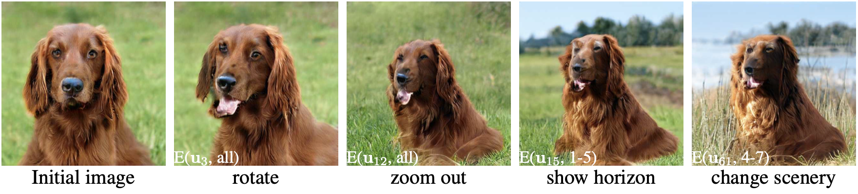
Irish Setter Interpolation - BigGAN
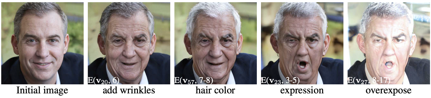
Man Face Interpolation - StyleGAN
Add a comment

Iterate on AI agents and models faster. Try Weights & Biases today.