Melanoma Detection Using Weights & Biases
In this article we look at how to identify melanoma in lesion images by extracting image features using a DenseNet121, image encodings, LightGBM, and Weights & Biases.
Created on August 4|Last edited on November 8
Comment
In this article, we give an overview of how to train a LightGBM classifier model to identify skin cancer from lesion images by extracting image features using a DenseNet121 and encoding them, and using Weights & Biases to track our experiments.
Table of Contents
What is Melanoma?Studying the dataExploratory Data AnalysisResizing the ImagesExtract features from ImagesTraining the Model and Hyperparameter OptimizationMaking PredictionsReferences
What is Melanoma?
Overview
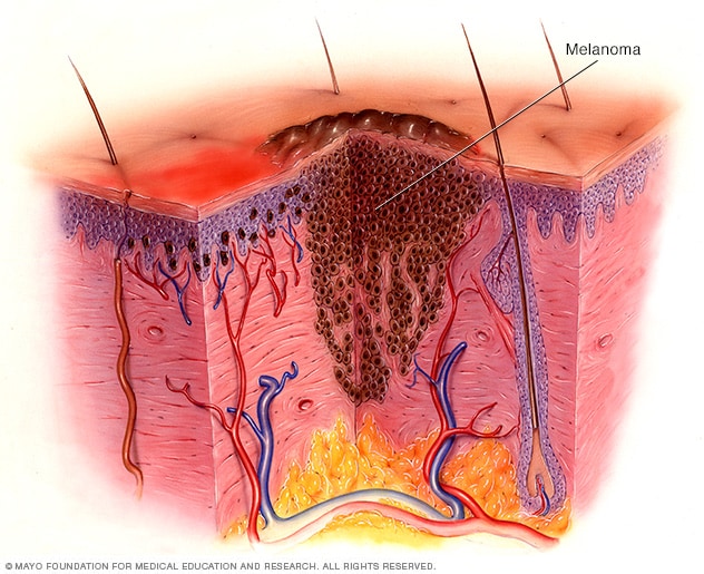
Melanoma, the most severe type of skin cancer, develops in the cells (melanocytes) that produce melanin — the pigment that gives your skin its color. Melanoma can also form in your eyes and, rarely, inside your body, such as in your nose or throat.
The exact cause of all melanomas is unclear, but exposure to ultraviolet (UV) radiation from sunlight or tanning lamps and beds increases your risk of developing melanoma. Limiting your exposure to UV radiation can help reduce your risk of melanoma.
The risk of melanoma seems to be increasing in people under 40, especially women. Knowing the warning signs of skin cancer can help ensure that cancerous changes are detected and treated before the cancer has spread. Melanoma can be treated successfully if it is detected early.
Symptoms
Melanomas can develop anywhere on your body. They most often develop in areas with exposure to the sun, such as your back, legs, arms, and face.
Melanomas can also occur in areas that do not receive much sun exposure, such as the soles of your feet, palms of your hands and fingernail beds. These hidden melanomas are more common in people with darker skin.
The first melanoma signs and symptoms often include a change in an existing mole, and the development of a new pigmented, or unusual-looking growth on your skin.
Melanoma does not always begin as a mole. It can also occur on otherwise normal-appearing skin.
Causes
Melanoma occurs when something goes wrong in the melanin-producing cells (melanocytes) that give color to your skin.
Usually, skin cells develop in a controlled and orderly way — healthy new cells push older cells toward your skin's surface, where they die and eventually fall off. However, when some cells develop DNA damage, new cells may begin to grow out of control and eventually form a mass of cancerous cells.
UV light does not cause all melanomas, especially those that occur in places on your body that do not receive sunlight exposure. This indicates that other factors may contribute to your risk of melanoma.
Studying the data
For complete code refer to my Kaggle Kernel.
The data required for this project can be accessed here. Interestingly, there are both tabular and image data. So, I will be extracting the features from Images(image encodings) and then combining it with the tabular data to make the predictions.
Below are some stats about the data:-
- Number of patients in the train set(A) is 2056 and number of patients in the test set(B): 690
- Number of images in the train set(C): 33126 and number of images in the test set(D): 10982
Now, let's study the distribution of data across the train and test sets.
Run set
1
Exploratory Data Analysis
Now that we have a sense of the data and what we are predicting, it would be better to explore a bit and find if there is something helpful hiding inside the data. If not, at least we can gather some insights for our knowledge.

The image above shows various differential diagnoses of pigmented skin lesions, by relative rates upon biopsy and malignancy potential, including "melanoma" at right.
Below are some insights gathered from the data:
Run set
1
Resizing the Images
In this section, I'll be defining the function to resize the images so that it becomes easier to extract features from them as we have a common ground. Also, I'll be plotting some random resized images from the train set and test set.
Full code in Kaggle Kernel
The Image size that I have chosen is 256x256.
This is the code I used to resize the images.
#Size to resize(256,256,3)img_size = 256def resize_image(img):old_size = img.shape[:2]ratio = float(img_size)/max(old_size)new_size = tuple([int(x*ratio) for x in old_size])img = cv2.resize(img, (new_size[1],new_size[0]))delta_w = img_size - new_size[1]delta_h = img_size - new_size[0]top, bottom = delta_h//2, delta_h-(delta_h//2)left, right = delta_w//2, delta_w-(delta_w//2)color = [0,0,0]new_img = cv2.copyMakeBorder(img, top, bottom, left, right,cv2.BORDER_CONSTANT, value=color)return new_imgdef load_image(path, img_id):path = os.path.join(path,img_id+'.jpg')img = cv2.imread(path)img = cv2.cvtColor(img, cv2.COLOR_BGR2RGB)new_img = resize_image(img)new_img = preprocess_input(new_img)return new_img
Extract features from Images
This entire process of extraction of features from images(image encodings) using DenseNet121 takes more than 2 hours. So, to save on time I have created this dataset. It contains all the extracted features and can be used by anyone.
Below the code is also available to get the image encodings.
img_size = 256batch_size = 16 #16 images per batchtrain_img_ids = df_train.image_name.valuesn_batches = len(train_img_ids)//batch_size + 1#Model to extract image featuresinp = Input((256,256,3))backbone = DenseNet121(input_tensor=inp, include_top=False)x = backbone.outputx = GlobalAveragePooling2D()(x)x = Lambda(lambda x: K.expand_dims(x,axis=-1))(x)x = AveragePooling1D(4)(x)out = Lambda(lambda x: x[:,:,0])(x)m = Model(inp,out)features = {}for b in tqdm_notebook(range(n_batches)):start = b*batch_sizeend = (b+1)*batch_sizebatch_ids = train_img_ids[start:end]batch_images = np.zeros((len(batch_ids),img_size,img_size,3))for i,img_id in enumerate(batch_ids):try:batch_images[i] = load_image(train_img_path,img_id)except:passbatch_preds = m.predict(batch_images)for i,img_id in enumerate(batch_ids):features[img_id] = batch_preds[i]train_feats = pd.DataFrame.from_dict(features, orient='index')#Save for future referencetrain_feats.to_csv('train_img_features.csv')train_feats.head()test_img_ids = df_test.image_name.valuesn_batches = len(test_img_ids)//batch_size + 1features = {}for b in tqdm_notebook(range(n_batches)):start = b*batch_sizeend = (b+1)*batch_sizebatch_ids = test_img_ids[start:end]batch_images = np.zeros((len(batch_ids),img_size,img_size,3))for i,img_id in enumerate(batch_ids):try:batch_images[i] = load_image(test_img_path,img_id)except:passbatch_preds = m.predict(batch_images)for i,img_id in enumerate(batch_ids):features[img_id] = batch_preds[i]test_feats = pd.DataFrame.from_dict(features, orient='index')test_feats.to_csv('test_img_features.csv')test_feats.head()
Later, using these features and the tabular data I'll train an LGBM classifier and make the predictions. The pre-trained NN used here is a DenseNet121. Per image, I'll be extracting 256 features for both the train and test set.

DenseNet Architecture

Normally DenseNet121 would output 1024 features after GlobalAveragePooling. To further narrow it down, I again pool 4 features each.
Training the Model and Hyperparameter Optimization
Finally, after fetching the image encodings, I'll combine them with the tabular data available (patient details like age, sex, diagnosis, e.t.c.) into a single dataframe. Eventually, I'll be using LGBM Classifier to classify the test data into benign/malignant.
Also, I'll perform Hyperparameter Optimization using Bayesian Optimization to find the most optimal hyperparameters for my LightGBM model.
Run set
50
Making Predictions
After getting the most optimal set of hyperparameters we are only left with just making the predictions on the test set.
#Hyparameters obtained through BOparams = {"num_leaves": 90,"max_depth": 6,"learning_rate": 0.002613,"bagging_freq": 12,"bagging_fraction": 0.9204,"feature_fraction": 0.9145,}#Making the Predictionsclf = LGBMClassifier(n_estimators=1000,**params)clf.fit(train[features],train['target'])sub_preds = clf.predict_proba(test[features])[:,1]#Preparing the submissionsubmission = pd.DataFrame({"image_name": df_test.image_name,"target": sub_preds})submission.to_csv('submission.csv', index=False)
The best score I have been able to achieve is 0.8953 on the test set.
I believe performing stacking by using different classifiers like Neural Network, KNeighborsClassifier, SVC e.t.c should definitely help in improving the score.
References
- I would like to thank Kaggle Grandmaster Dieter for sharing this awesome kernel to extract features from images using a pre-trained NN.
Add a comment
Tags: Intermediate, Computer Vision, Object Detection, Experiment, DenseNet, Panels, Plots, Kaggle, Health Care

Iterate on AI agents and models faster. Try Weights & Biases today.