Part 2: Deep Representations, a Way Towards Neural Style Transfer
This article is the second part of two, and it provides a top-down approach to conceiving neural style transfer using Weights & Biases.
Created on September 2|Last edited on November 6
Comment
This is the second part of the two-part series on Neural Style Transfer. If you have arrived here from the first part, you already know how content representations are learned, how to visualize the deep embeddings of a convolutional neural network, and are also familiar with amalgamation.
Style Transfer for each layer of VGG16
Table of Contents
Style Representation
Part 1 focused on content representation and explored how our white noise image captures most of the non-abstract concrete features present in the image. For example, when choosing a dog picture as our content image, we need our generated image to contain the dog and its associated features.
This is where the crossroads of content representation and style representation lie. For style representation, we want to learn the artistic texture of the image, but we also do not want any kind of content from the style image to leak into our generated picture.
An excerpt from the Neural Style Transfer paper:
To obtain a representation of the style of an input image, we use a feature space designed to capture texture information. It consists of the correlations between the different filter responses, where the expectation is taken over the spatial extent of the feature maps. These feature correlations are given by the Gram Matrix where is the inner product between the vectorised feature maps and in layer
Consider the activation maps of a Conv layer. Each map in the layer is a feature that has been extracted from the image. In a particular layer, we can compute the correlation between each of these extracted features. This intuitively conveys a star aspect of style representation. If we encode the correlation between different activation maps (the extracted features), we encode the abstract style that each of the kernels in that layer encodes.
We have taken an elementary example to make sense of the Gram Matrix of a Conv layer. For simplicity, we have taken 4 activation maps in a layer. The table on the right conveys the correlation between each of the 4 activation maps. The maps' different colors can be thought of as the different features of the image that it encodes. The correlation conveys how similar or dissimilar a pair of feature map is.
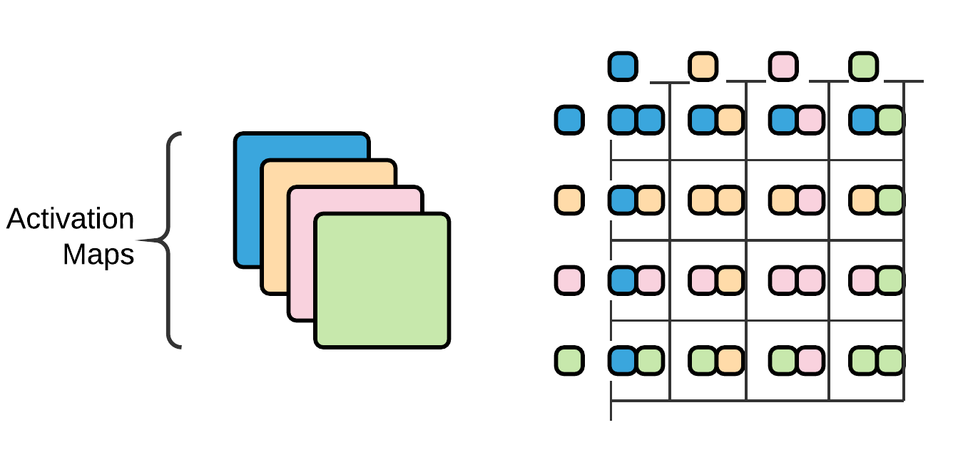
Example Gram Matrix
The efficiency of computing Gram Matrices: Visualize a vector of size (224, 224, 64). Reshaping it by unrolling its height and width would lead to a matrix of size (224x224, 64). The Gram Matrix of the layer would comprise the product. This leads to a resultant matrix of size (64,64).
This matrix represents the correlation of the original vector between its features by giving up values for pairs of outer products. From this representation, we can see which of the outer products fire together, establishing a correlation. Essentially, the values of a gram matrix show similarities between activation maps.
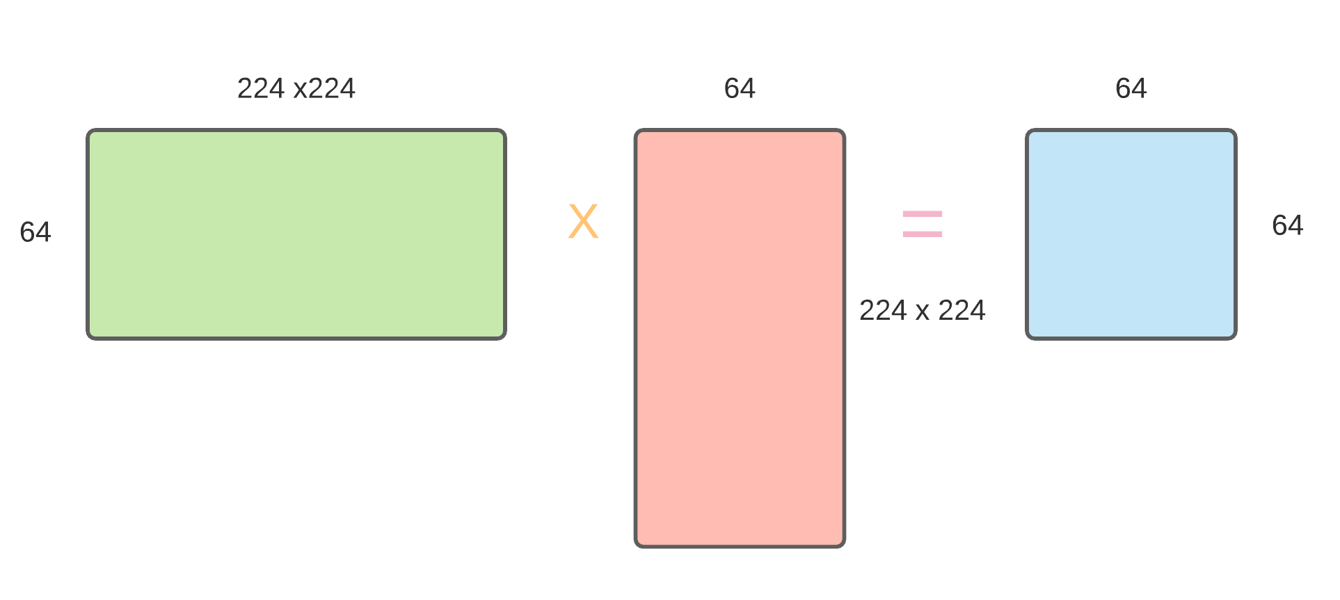
The matrix multiplication for Gram Matrix
In other words, instead of raw activations, we want the Gram matrices from our activation outputs. The losses generated by these gram matrices are backpropagated, and the pixels of our noisy image are changed. These gram matrices are spatially invariant and are used to analyze which pair of outer products activate together.
Using the feature correlation of multiple layers results in a stationary output that vividly captures the image's artistic abstractness but prevents any global-scale concrete features from appearing in our generated image.

The gram matrix losses
Since it connects the abstract idea (an inner product) with a concrete computation, the authors chose this as their means of unravelling the secrets of texture transfer.
In the panel below, we would look at the style representation coded in each layer of the normalized pre-trained VGG16 model.
Run set
5
We can see that each layer encodes some style from the style image. What if we aggregate the encoded styles from each layer?
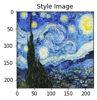
In this panel, we would see exactly that. The style image remains the same. The style representations have been combined with an equal weight of representation to each layer in the VGG16 model.
Run set
1
Neural Style Transfer
When we combine the content and style representation discussed in the earlier sections, we get our ultimate outcome; Neural Style Transfer.
To transfer the style of artwork onto a photograph , we synthesize a new image that simultaneously matches the content representation of and the style representation of . However, there is a BIG catch. Several things come into effect when we have two losses (Style loss and content loss) working together to reduce the total loss.
First, let us mathematically define our loss:
The coefficients and also play an essential role, which we shall soon get into.
Let us visualize the concept in our minds. We have our white noise image . When dealing with just the content representation, there is only a single loss determining how the noisy image will change. As the loss curve decreases, we see our required content slowly appearing in our noisy image. No problem!
Let us visualize our noisy image again. This time we are only representing the style from another image. Just as last time, as our single style loss decreases, we see abstract representations of style appearing on our noisy image. Still not a problem.
Now, what happens when we combine them and make them work in unison to achieve our ultimate goal of Neural Style transfer? Let us see for ourselves:
Run set
5
The Game of Losses
As mentioned earlier, the individual losses (content loss and style loss) have no problem converging on their own. The problem starts to emerge when both the losses are taken together. In the algorithm of Neural Style Transfer, the content loss helps in extracting the content, whereas the style loss helps in imprinting the style. As it happens, in each epoch, the white noise image updates in correspondence to the style loss and the content loss. With the update of any one of the losses, the gradients change quite a bit for the next iteration. The mutual loss makes Neural Style Transfer a little hard to guess and understand.
As stated above, there are two coefficients in the total loss equation, and , respectively. is the coefficient of content loss, while corresponds to the coefficient of the style loss. These coefficients help in controlling the amount of style and content in the mutual setup.
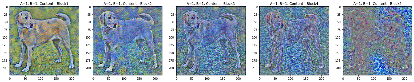
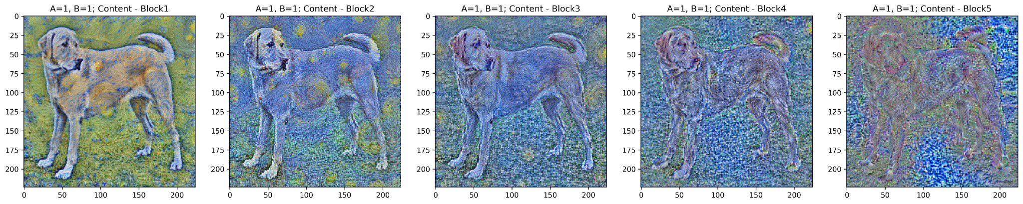
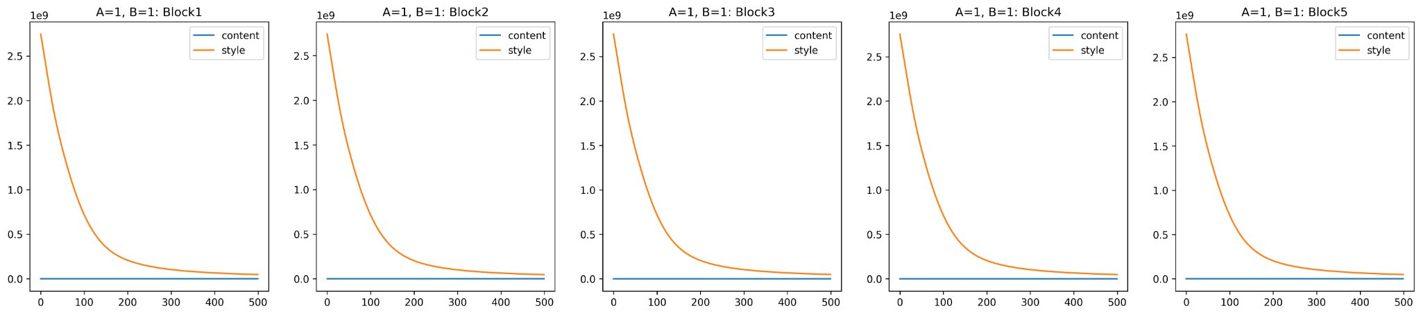
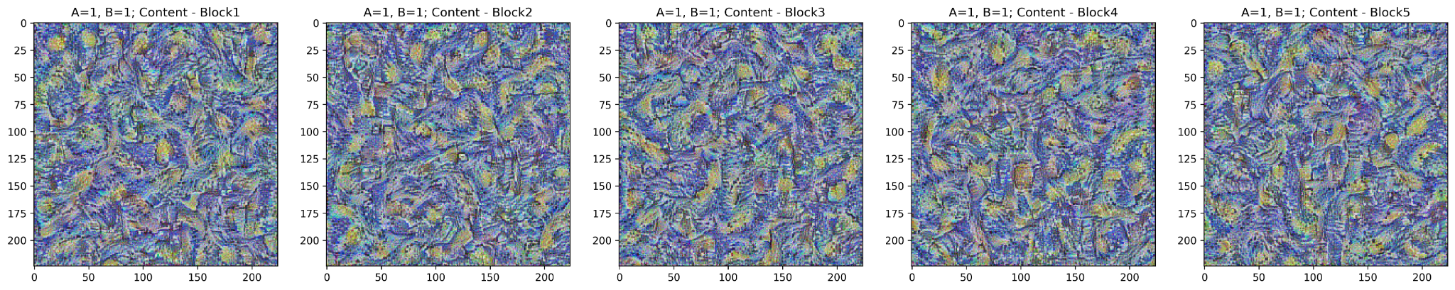
=1, =1:
Here, this is the vanilla setup, where we want both the losses to be playing their own game without outweighing each other. In this vanilla mutual setup, both the losses do not converge smoothly. There are times when the content loss saturates or acknowledges a little bump along the way. The loss curves directly imply the images that are generated.
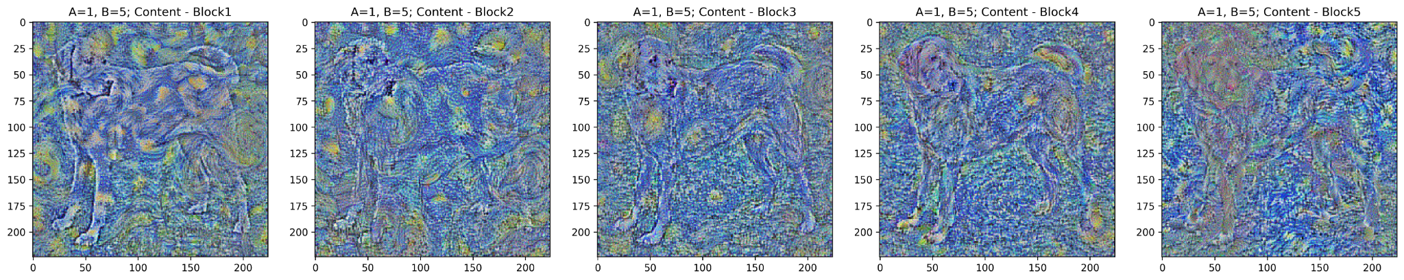
=1, =5:
Here . Here the style overpowers the content. This is quite evident from the loss curves and the generated images as well. The content does get its representation, but somewhere down the epoch, style wins its battle.
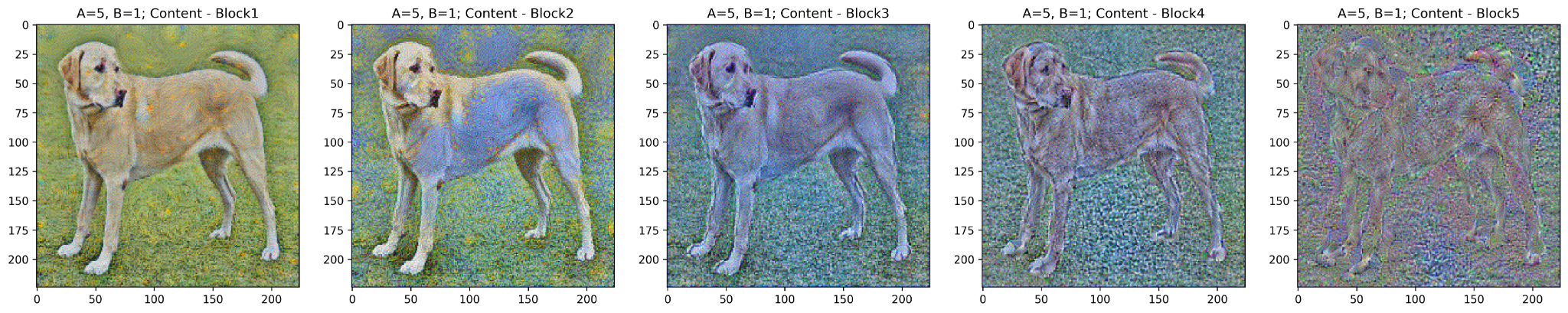
=5, =1:
Here the content overpowers the style. In the first layer, the style does not even find any representation as seen in the generated picture.
This section shows why one needs to play with the mutual loss setup to understand how Neural Style Transfer works. We would also suggest the readers look into different images and look at the mutual loss. The alpha and beta are subject to change from each content image and style image.
Unnormalized VGG16
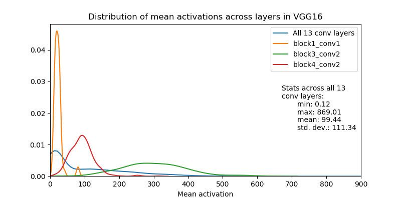
The picture above is of the distribution of the activation maps of the VGG16 pretrained model. It is evident here that the activation maps are not normalized. This phenomenon is because the VGG16 model does not have any normalization layers, and the idea of normalization came in later.
The authors of Neural Style Transfer argue that with an unnormalized VGG16, the mutual loss and the generated images are tough to interpret. The scale of loss for each layer does not match. Due to this mismatch, the coefficients of loss seems to be varying intrinsically.
To better understand the problem, below, we will look at the mutual loss and analyze the problem.
The loss curves make it quite evident that the unnormalized VGG16 model would make the training a lot more complicated. The activations and the gram matrix are out of scale in this process. This directly implies that the unnormalized VGG16 model has an intrinsic value of and , which is unknown to us. We would first need to guess the coefficients and then scale the coefficients properly to get the desired Artistic Neural Style Transfer image.
Conclusion
That is the end of the two-part series of Neural Style Transfer. We hope the reader can now make sense of the steps involved in the whole process. Conceiving the idea of Gram Matrix is what makes the research paper to stand out.
Some of the topics we could not include in the report:
- Using a different training set other than ImageNet.
- Using a different tool for style representation.
- Using a different architecture, one with Batch-Normalization.
We encourage the readers to take one of the topics and fire up an experiment.
Reach the authors
| Name | Github | |
|---|---|---|
| Aritra Roy Gosthipaty | @ariG23498 | @ariG23498 |
| Devjyoti Chakraborty | @cr0wley-zz | @Cr0wley_zz |
Add a comment
Tags: Intermediate, Computer Vision, GenAI, Experiment, Research, CNN, Github, Panels, Plots, Slider, ImageNet

Iterate on AI agents and models faster. Try Weights & Biases today.