
Block-NeRF: Scalable Large Scene Neural View Synthesis
Representing large city-scale environments spanning multiple blocks using Neural Radiance Fields
Created on February 28|Last edited on March 14
Comment
Introduction
In 2020, the paper NeRF: Representing Scenes as Neural Radiance Fields for View Synthesis presented a novel method for synthesizing novel views of complex scenes by optimizing an underlying continuous volumetric scene function using a sparse set of input views. But the question that we ask ourselves today is whether this method can be scaled to represent extremely large or complicated scenes. Essentially:
Is it possible to represent a city-scale scene spanning multiple blocks using Neural Radiance Fields?
This is the problem the authors of the paper Block-NeRF: Scalable Large Scene Neural View Synthesis attempt to solve. They use images captured from multiple different trips in an autonomous vehicle to construct Block-NeRFs (3D representations of a large and complex scene at the scale of a single city block). Once constructed, we're no longer confined to the path of the vehicle traversed and can explore the scene from new viewpoints outside the vehicles' point of view.
The authors demonstrate this novel and large-scale view synthesis approach by constructing the Alamo Square, a square kilometer residential neighborhood in San Francisco famous for the Painted Ladies (and the title sequence of the sitcom Full House). This area is represented by a grid of 35 Block-NeRFs built from 2.8 million images collected over a period of over 3 months resulting in the largest neural scene representation till date. Here's the map of Alamo Square and a few sample reconstructed views:
Block-NeRF can update individual blocks of the environment without retraining on the entire scene, as demonstrated by the reconstructed views in the aforementioned panel from the same block in the month of June (when the building was under construction) and the same view in the month of September (when the construction was complete).
💡
A Brief Overview of NeRF
NeRF or Neural Radiance Fields is a method proposed by the paper NeRF: Representing Scenes as Neural Radiance Fields for View Synthesis that achieves SoTA results for synthesizing novel views of complex scenes by optimizing an underlying continuous volumetric scene function using a sparse set of input views. It is a coordinate-based neural scene representation optimized through a differentiable rendering loss to reproduce the appearance of a set of input images from known camera poses. Importantly, after optimization, the NeRF model can be used to render previously unseen viewpoints.
Scene Representation Architecture
The NeRF scene representation is a pair of multilayer perceptrons (MLPs). The first MLP takes in a 3D position x and outputs volume density and a feature vector. This feature vector is concatenated with a 2D viewing direction and fed into the second MLP which outputs an RGB color . This architecture ensures that the output color can vary when observed from different angles, allowing NeRF to represent reflections and glossy materials, but that the underlying geometry represented by is only a function of position.
To enable the NeRF MLPs to represent higher frequency detail, the inputs and are each preprocessed by a component-wise sinusoidal positional encoding given by
...where, is the number of levels of positional encoding.
The Positional Encoding strategy is proposed by the paper Fourier Features Let Networks Learn High Frequency Functions in Low Dimensional Domains.
💡

The NeRF MLPs as a unified architecture. Source: Figure 7 from the paper NeRF: Representing Scenes as Neural Radiance Fields for View Synthesis.
View Synthesis
Each pixel in an image corresponds to a ray propagating through the 3D space given by where the ray parameter is a real number. In order to calculate the color of the ray , NeRF randomly samples distances along the ray and passes the points and direction through its MLPs to calculate and . The resulting output color is given by
...where
- is the transmittance of the point given by
- is the change in the parameter or
Transmittance represents how visible a point is from a particular input camera. Points in free space or on the surface of the first intersected object will have transmittance near 1, and points inside or behind the first visible object will have transmittance near 0. If a point is seen from some viewpoints but not others, the regressed transmittance value will be the average over all training cameras and lie between zero and one, indicating that the point is partially observed.
💡
Multi-scale Representations by Mip-NeRF
NeRF’s MLP takes a single 3D point as input. However, this ignores both the relative footprint of the corresponding image pixel and the length of the interval along the ray containing the point, resulting in aliasing artifacts when rendering novel camera trajectories. Mip-NeRF solves this issue by using the projected pixel footprint to sample conical frustums along the ray rather than intervals. In order to feed these frustums into the MLP, mip-NeRF approximates each of them as Gaussian distributions with parameters , and replaces the positional encoding with its expectation over the input Gaussian referred to as an integrated positional encoding given by
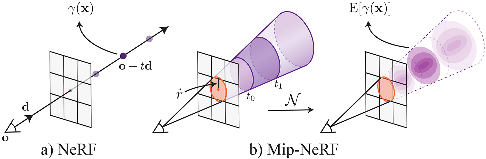
Mip-NeRFs use projected pixel footprint to sample conical frustums along the ray. Source: https://jonbarron.info/mipnerf/
Novel View Synthesis by Block-NeRF
The Task at Hand: Given a set of input images of a scene and their respective camera poses, novel view synthesis seeks to render observed scene content from previously unobserved viewpoints, allowing a user to navigate through a recreated environment with high visual fidelity.
In other words: can we use a library of images to construct vantage points not in the images themselves?
Shortcomings of Geometry-Based Image Reprojection
Many approaches to view synthesis start by applying traditional 3D reconstruction techniques to build a point cloud or triangle mesh representing the scene. This geometric “proxy” is then used to reproject pixels from the input images into new camera views, where they are blended by heuristic or learning-based methods (such as Deep Blending for Free-Viewpoint Image-Based-Rendering and Free View Synthesis). Such methods that rely on geometry proxies are limited by the quality of the initial 3D reconstruction, which hurts their performance in scenes with complex geometry or reflectance effects.
Shortcomings of Volumetric Scene Representations
Several recent works in view synthesis have focused on unifying reconstruction as well as rendering and learning this pipeline end-to-end, typically using a volumetric scene representation.
For example, methods for rendering small baseline view interpolation such as DeepStereo and Stereo Magnification often use feed-forward networks to learn a mapping directly from input images to an output volume while Methods such as Neural Volumes that target larger-baseline view synthesis run a global optimization overall input images to reconstruct every new scene.
NeRF combines this single scene optimization setting with a neural scene representation capable of representing complex scenes much more efficiently than a discrete 3D voxel grid. However, its rendering model scales very poorly to large-scale scenes in terms of compute resources. Follow-up work has proposed making NeRF more efficient by partitioning space into smaller regions, each containing its own lightweight NeRF network. However, these network ensembles must be trained jointly, limiting their flexibility.
Overcoming these Challenges using Block-NeRF
- The authors of Block-NeRF built their implementation on top of Mip-NeRF, which, as we discussed previously, improves the aliasing issues that hurt NeRF’s performance in scenes where the input images observe the same scene from many different distances.
- The authors also incorporate techniques from NeRF in the Wild or NeRF-W, which adds a latent code per training image to handle inconsistent scene appearance when applying NeRF to landmarks from the Photo Tourism dataset.
- Although NeRF-W creates a separate NeRF for each landmark from thousands of images, the Block-NeRF approach combines many NeRFs to reconstruct a coherent large environment from millions of images.
- Block-NeRF also incorporates a learned camera pose refinement which has been explored in previous works.
Some NeRF-based methods use segmentation data to isolate and reconstruct static or moving objects (such as cars or people) across video sequences. Since the focus of Block-NeRF is primarily on reconstructing the environment itself, the dynamic objects are simpley masked out during training.
💡
The Block-NeRF Approach
Training a single NeRF does not scale when trying to represent scenes as large as cities. To overcome this challenge, the authors of Block-NeRF propose splitting the environment into a set of Block-NeRFs that can be independently trained in parallel and composited during inference.
This independence enables the ability to expand the environment with additional Block-NeRFs or update blocks without retraining the entire environment. Relevant Block-NeRFs are dynamically selected for rendering, which are then composited in a smooth manner when traversing the scene.
To aid with this compositing, the appearances codes are optimized to match lighting conditions and use interpolation weights computed based on each Block-NeRF’s distance to the novel view.
Block Size and Placement
The individual Block-NeRFs should be arranged to collectively ensure full coverage of the target environment. Typically a single Block-NeRF is placed at each intersection, covering the intersection itself and any connected street 75% of the way until it converges into the next intersection, resulting in a 50% overlap between any two adjacent blocks on the connecting street segment, making appearance alignment easier between them. This process ensures that the block size is variable, i.e, additional blocks may be introduced as connectors between intersections wherever necessary. The authors ensure that the training data for each block stay exactly within its intended bounds by applying a geographical filter using basic map data such as OpenStreetMap.
For a given scene, it's split into multiple Block-NeRFs, each trained on data within some radius (denoted by the dotted orange line in the following figure) of a specific Block-NeRF origin coordinate (the orange dots in the following figure). In order to render a target view in the scene, the visibility maps are computed for all of the NeRFs within a given radius. Block-NeRFs with low visibility are discarded (bottom Block-NeRF) and the color output is rendered for the remaining blocks. The renderings are then merged based on each block origin’s distance to the target view.
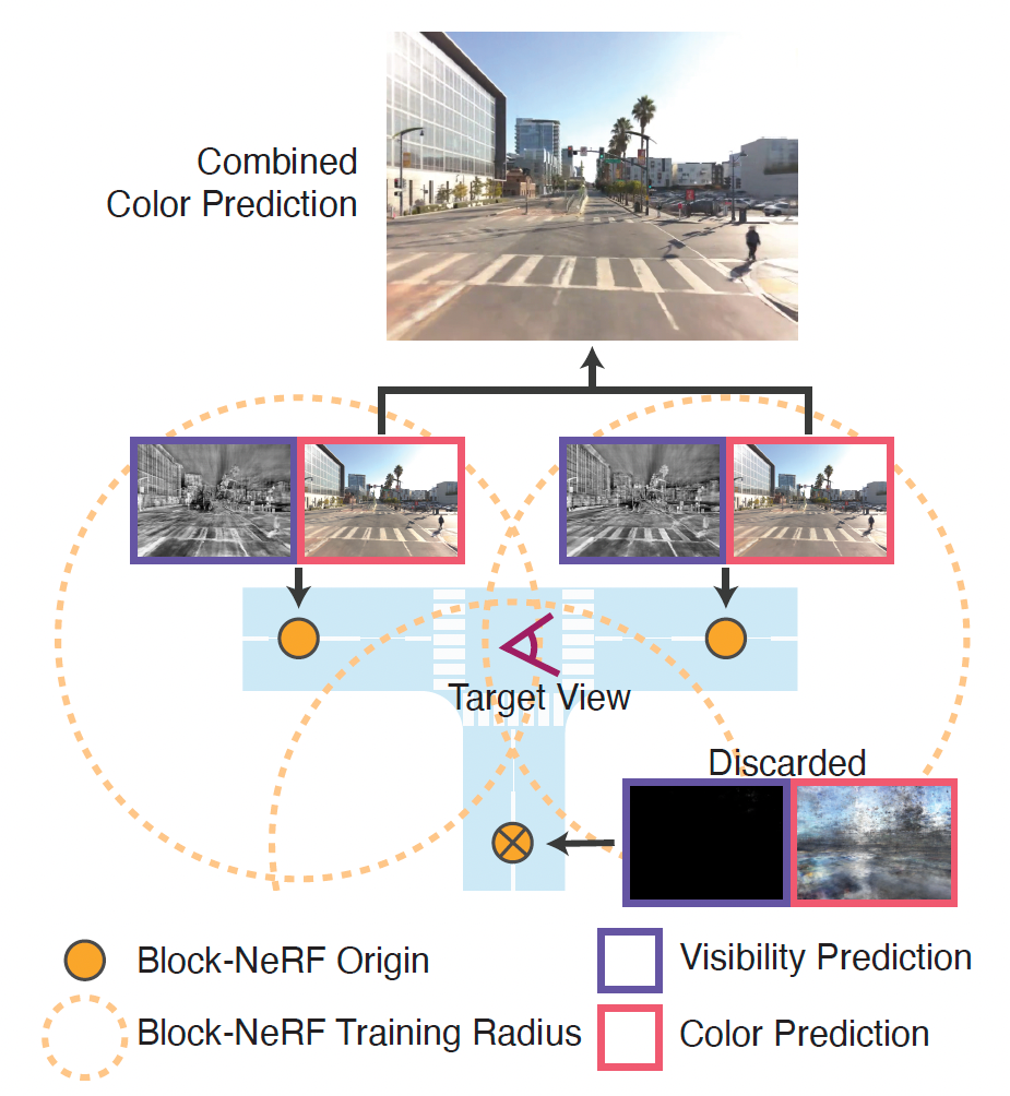
Source: Figure 2 from the paper.
Note that it's possible to follow other placement heuristics as well, as long as the entire environment is covered by at least one Block-NeRF. For example, for some of the experiments performed by the authors blocks were placed along a single street segment at uniform distances and define the block size as a sphere around the Block-NeRF Origin, as shown in the aforementioned figure.
💡
Training Individual Block-NeRFs
As mentioned before, Block-NeRF is an extension of the model presented in Mip-NeRF. Similar to Mip-NeRF, the first MLP predicts the density for a position in space. The network also outputs a feature vector that is concatenated with viewing direction , the exposure level, and an appearance embedding. These are fed into a second MLP that outputs the color for the point. Additionally, a visibility network is also trained to predict whether a point in space was visible or not.

Source: Figure 3 from the paper
Appearance Embeddings
Given that different parts of our data may be captured under different environmental conditions, the authors follow NeRF-W and use Generative Latent Optimization to optimize per-image appearance embedding vectors. This allows the NeRF to explain away several appearance-changing conditions, such as varying weather and lighting. These appearance embeddings can additionally be manipulated to interpolate between different conditions observed in the training data, such as cloudy versus clear skies or day and night.
Learned Pose Refinement
Although we assumed that the camera poses are provided, it is found advantageous to learn regularized pose offsets for further alignment. Pose refinement has been explored in previous NeRF based models (such as BARF, A-NeRF, Nerf– and iNeRF) in which the pose offsets are learned per driving segment and include both a translation and a rotation component. These offsets are jointly optimized with the NeRF itself, significantly regularizing the offsets in the early phase of training to allow the network to first learn a rough structure prior to modifying the poses.
Exposure Input
Training images may be captured across a wide range of exposure levels, which can impact NeRF training if left unaccounted for. The authors that feeding the camera exposure information to the appearance prediction part of the model allows the NeRF to compensate for the visual differences. Specifically, the exposure information is processed as where is a sinusoidal positional encoding with 4 levels, and is a scaling factor (the authors use 1000 in practice) and z = shutter_speed * analog_gain / t.
Transient Objects
While the Block-NeRF approach accounts for variation in appearance using the appearance embeddings, it is assumed that the scene geometry is consistent across the training data. Any movable objects, such as cars and pedestrians typically violate this assumption. Hence, the authors use a Panoptic DeepLab, a panoptic segmentation model to produce masks of common movable objects, and ignore masked areas during training. While this does not account for changes in otherwise static parts of the environment, such as buildings under construction, it accommodates most of the common types of geometric inconsistencies.
Visibility Prediction
While merging multiple Block-NeRFs, it can be useful to know whether a specific region of space was visible to a given NeRF during training. The authors extend Block-NeRF with an additional MLP that is trained to learn an approximation of the visibility of a sampled point. For each sample along a training ray, takes in the location and view direction and regresses the corresponding transmittance of the point. The model is trained alogside which provides the supervision. The visibility prediction in Block-NeRF is similar to the Visibility Fields as proposed by the paper NeRV: Neural Reflectance and Visibility Fields for Relighting and View Synthesis, although instead of using an MLP to predict visibility to environment lighting for the purpose of recovering a relightable NeRF model, the Block-NeRF architecture predicts the visibility to the training rays.
The visibility network is small and can be run independently from the color and density networks. This proves useful when merging multiple NeRFs since it can help to determine whether a specific NeRF is likely to produce meaningful outputs for a given location. The visibility predictions can also be used to determine locations to perform appearance matching between two NeRFs.
Merging Multiple Block-NeRFs
Block-NeRF Selection
A given environment can be composed of an arbitrary number of Block-NeRFs. For efficiency, we utilize two filtering mechanisms to only render relevant blocks for the given target viewpoint. Only the Block-NeRFs that are within a set radius of the target viewpoint. Additionally, for each of these candidates, the associated visibility is also computed and if the mean visibility is below a certain threshold, that particular Block-NeRF is discarded. Visibility can be computed quickly because its network is independent of the color network, and it does not need to be rendered at the target image resolution. After filtering, there are typically one to three Block-NeRFs left to merge.
Block-NeRF Compositing
Color images are rendered from each of the filtered Block-NeRFs and interpolated between them using inverse distance weighting between the camera origin c and the centers of each Block-NeRF. Specifically, the authors calculate the respective weights as
...where, is a hyperparameter that influences the rate of blending between Block-NeRF renders. The interpolation is done in 2D image space and produces smooth transitions between Block-NeRFs.
Appearance Matching
The appearance of our learned models can be controlled by an appearance latent code after the Block-NeRF has been trained. These codes are randomly initialized during training and therefore the same code typically leads to different appearances when fed into different Block-NeRFs. This is undesirable when compositing as it may lead to inconsistencies between views. Given a target appearance in one of the Block-NeRFs, the aim is to match its appearance in the remaining blocks. In order to accomplish this, first, a 3D matching location is selected between pairs of adjacent Block-NeRFs. The visibility prediction at this location should be high for both Block-NeRFs.
Given the matching location, the Block-NeRF network weights are frozen and only the appearance codes of the target are optimized in order to reduce the loss between the respective are renderings. This optimization is quick, converging within 100 iterations. Although it does not necessarily yield perfect alignment, this procedure aligns most global and low-frequency attributes of the scene, such as time of day, color balance, and weather, which is a prerequisite for successful compositing. The optimized appearance is iteratively propagated through the scene. Starting from one root Block-NeRF, the appearance of the neighboring ones is optimized, and continue the process from there. If multiple blocks surrounding a target Block-NeRF have already been optimized, then each of them is considered when computing the loss.
Results and Experiments
San Fransisco Alamo Square Dataset
The authors select San Francisco’s Alamo Square neighborhood as the target area for the scalability experiments. The dataset spans an area of approximately 960m x 570m, and was recorded in June, July, and August of 2021. This dataset is divided into 35 Block-NeRFs each of which was trained on data from 38 to 48 different data collection runs, adding up to a total driving time of 18 to 28 minutes each. After filtering out some redundant image captures (such as stationary captures), each Block-NeRF is trained on between 64575 to 108216 images. The overall dataset is composed of 13.4 h of driving time sourced from 1330 different data collection runs, with a total of 2818745 training images.
San Francisco Mission Bay Dataset
The authors choose San Francisco’s Mission Bay District as the target area for the baseline, block size, and placement experiments. Mission Bay is an urban environment with challenging geometry and reflective facades. A long stretch on Third Street was identified with far-range visibility, making it an interesting test case. Notably, this dataset was recorded in a single capture in November 2020, with consistent environmental conditions allowing for simple evaluation. This dataset was recorded over 100s, in which the data collection vehicle traveled 1.08km and captured 12000 total images from 12 cameras.
Reconstructions from San Francisco
Model Ablations
The authors perform ablation studies on model modifications on a single intersection from the Alamo Square dataset. The Peak Signal-to-Noise Ratio (PSNR), Structural Similarity (SSIM), and Learned Perceptual Image Patch Similarity (LPIPS) metrics for the test image reconstructions are reported in the following panel.
Observations from Ablation Study
- We can observe that Mip-NeRF alone fails to properly reconstruct the scene and is prone to adding non-existent geometry and cloudy artifacts to explain the differences in appearance.
- When Block-NeRF is not trained with appearance embeddings, these artifacts are still present. If our method is not trained with pose optimization, the resulting scene is blurrier and can contain duplicated objects due to pose misalignment.
- The exposure input marginally improves the reconstruction but more importantly provides us with the ability to change the exposure during inference.
The test images are split in half vertically, with the appearance embeddings being optimized on one half and tested on the other.
💡
Block-NeRF Size and Placement
The authors show the comparison of different numbers of Block-NeRFs for reconstructing the Mission Bay dataset in the following table. It is ensured that each pair of adjacent blocks overlaps by 50% and compare other overlap percentages in the supplement. All the evaluation was done on the same set of held-out test images spanning the entire trajectory.
Observations from the Size and Placement Comparison
- We observe that increasing the number of models improves the reconstruction metrics.
- In terms of computational expense, parallelization during training is trivial as each model can be optimized independently across devices. At inference, rendering Block-NeRFs near the target view is required.
- Depending on the scene and NeRF layout, typically between one to three NeRFs are rendered.
- Splitting the scene into multiple lower capacity models can reduce the overall computational cost as not all of the models need to be evaluated.
Interpolation Methods
Observations from Different Interpolation Methods
- The simple method of only rendering the nearest Block-NeRF to the camera requires the least amount of compute but results in harsh jumps when transitioning between blocks.
- These transitions can be smoothed by using simple Inverse Distance Weighting (IDW) in image space between the camera and Block-NeRF centers. An IDW power of 4 is used for the Alamo Square renderings and a power of 1 for the Mission Bay renderings.
- The authors also explored a variant of IDW where the interpolation was performed over projected 3D points predicted by the expected Block-NeRF depth. This method suffers when the depth prediction is incorrect, leading to artifacts and temporal incoherence.
- The authors also experiment with weighing the Block-NeRFs based on per-pixel and per-image predicted visibility. This produces sharper reconstructions of further-away areas but is prone to temporal inconsistency.
Limitations and Future Work
Limitations
- The proposed method handles transient objects by filtering them out during training via masking using a segmentation algorithm. If objects are not properly masked, they can cause artifacts in the resulting renderings. For example,
- the shadows of cars often remain, even when the car itself is correctly removed.
- Vegetation also breaks this assumption as the foliage changes seasonally and moves in the wind; this results in blurred representations of trees and plants.
- Temporal inconsistencies in the training data, such as construction work, are not automatically handled and require the manual retraining of the affected blocks.
- The inability to render scenes containing dynamic objects currently limits the applicability of Block-NeRF towards closed-loop simulation tasks in robotics.
Future Works to Overcome the Limitations
- In the future, these issues could be addressed by learning transient objects during the optimization (as demonstrated by NeRF-W) or directly modeling dynamic objects (as demonstrated by the paper Neural Scene Graphs for Dynamic Scenes and Learning Object-Compositional Neural Radiance Field for Editable Scene Rendering). In particular, the scene could be composed of multiple Block-NeRFs of the environment and individual controllable object NeRFs.
- In the case of Block-NeRF, distant objects in the scene are not sampled with the same density as nearby objects which leads to blurrier reconstructions. This is an issue with sampling unbounded volumetric representations. Techniques proposed in NeRF++ and concurrent Mip-NeRF 360 could potentially be used to produce sharper renderings of distant objects.
- In many applications, real-time rendering is key, but NeRFs are computationally expensive to render (up to multiple seconds per image). Several NeRF caching techniques or a sparse voxel grid could be used to enable real-time Block-NeRF rendering. Similarly, multiple concurrent works have demonstrated techniques to speed up the training of NeRF style representations by multiple orders of magnitude.
Societal Impact
Methodological
The proposed method inherits the heavy compute footprint of NeRF models and the authors propose to apply them at an unprecedented scale (hitherto undreamt of). It also unlocks new use-cases for neural renderings, such as building detailed maps of the environment, which could cause more widespread use in favor of less computationally involved alternatives. Depending on the scale this work is being applied at, its compute demands can lead to or worsen environmental damage if the energy used for compute leads to increased carbon emissions. As we have already mentioned in the previous section, the authors foresee further work, such as caching methods, that could reduce the compute demands and thus mitigate the environmental damage.
Application
As per the experiments conducted by the authors, the proposed method was applied to real city environments. During the data collection efforts for this paper, the authors were careful to blur faces and sensitive information, such as license plates, and limited our driving to public roads. Future applications of this work might entail even larger data collection efforts, which raises further privacy concerns. While detailed imagery of public roads can already be found on services like Google Street View, the proposed methodology could promote repeated and more regular scans of the environment. Several companies in the autonomous vehicle space are also known to perform regular area scans using their fleet of vehicles, however, some might only utilize LiDAR scans which can be less sensitive than collecting camera imagery.
Conclusion
Block-NeRF is a novel method that is able to reconstruct arbitrarily large (city-scaled) environments using Neural Radiance Fields or NeRFs. The efficacy of the approach is demonstrated by the authors of the respective paper by building an entire neighborhood in San Francisco from 2.8M images, forming the largest neural scene representation to date. This immense scale of reconstruction using NeRFs is accomplished by splitting our representation into multiple blocks that can be optimized independently. At such a scale, the data collected will necessarily have transient objects and variations in appearance, which are accounted for by modifying the underlying NeRF architecture.
Similar Posts
NeRF – Representing Scenes as Neural Radiance Fields for View Synthesis
Generating Digital Painting Lighting Effects via RGB-space Geometry
Exploring the paper "Generating Digital Painting Lighting Effects via RGB-space Geometry" in which the authors propose an image processing algorithm to generate digital painting lighting effects from a single image.
3D Image Inpainting With Weights & Biases
In this article, we take a look at a novel way to convert a single RGB-D image into a 3D image, using Weights & Biases to visualize our results.
Creating 3D Meshes with Neural ODEs
Diffeomorphic Genus-0 Mesh Generation using Neural ODEs
Add a comment

Iterate on AI agents and models faster. Try Weights & Biases today.