
The rise of large language models promises a revolution in AI, but deploying them reliably in the real world introduces a complex new frontier: LLMOps. If you’ve attempted to manage LLMs with traditional MLOps tools, you’ve likely discovered they can fall short. Why? Because LLMs simply don’t play by the old rules.
Traditional machine learning operations were built for a different era. These systems thrive on deterministic outputs from models trained on fixed datasets. They track prediction accuracy against clear ground-truth labels, and the performance metrics map directly to predictable business outcomes.
LLM systems, however, elegantly (or sometimes chaotically) violate every one of these assumptions. A single user query can trigger a complex chain of events involving vector database retrieval, multiple reasoning steps, calls to external APIs, and the synthesis of a final, coherent response. What’s more, identical inputs can produce different outputs due to the stochastic nature of these models. And unfortunately, quality metrics are difficult to quantify. Factors like creativity, tone, and the ability to address underlying user intent often matter far more than simple binary correctness. Standard dashboards, designed for traditional ML, miss these crucial dimensions entirely.
The biggest headaches often emerge from the persistent gap between development and production environments. Models trained on pristine, curated datasets frequently behave differently when faced with the messy reality of user queries. External dependencies can change without warning, and user expectations continuously shift as competitors release new features. Without specialized instrumentation and monitoring, these critical changes often surface only through the unfortunate avenue of user complaints.
This article presents a robust framework for continuous LLM evaluation, a system designed to bridge this gap by connecting granular development traces directly to real-time production monitoring. We’ll start by exploring the unique challenges and new forms of degradation LLMs face. Then, we’ll demonstrate these problems through a controlled experiment on retrieval drift before diving into a practical tutorial on implementing a complete observability loop with Weights & Biases.
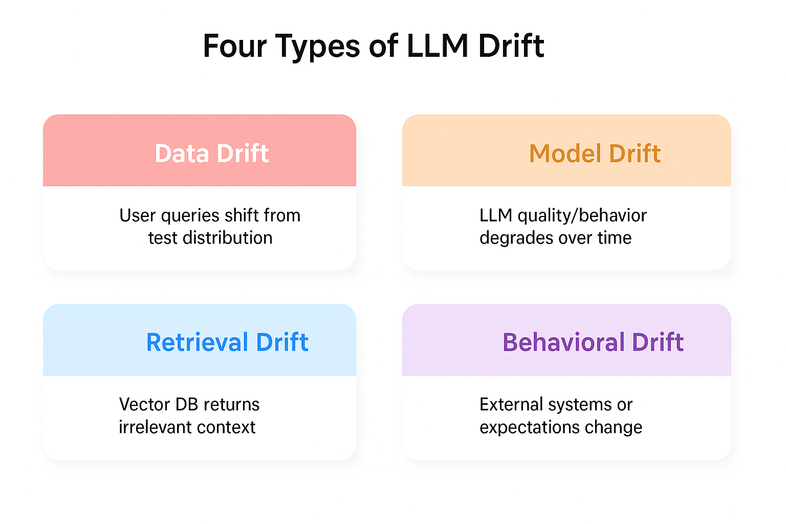
“Figure 1: Four distinct types of drift in production LLM systems, each requiring different monitoring approaches.”
To truly illustrate the insidious nature of retrieval drift, let’s dive into a controlled experiment using LangChain’s public documentation. Our goal is to clearly show how degraded retrieval impacts the quality of an LLM’s response long before aggregate metrics typically flag a problem.
To illustrate, we constructed a simple RAG system. For retrieval, we used sentence-transformers, and for generation and evaluation, we employed Anthropic’s claude-sonnet-4-20250514. The core query we aimed to answer was: “How do I create a basic chain in LangChain? Provide a simple code example.”
We created two distinct document pools for retrieval:
Healthy Pool: Contains three current LangChain documentation pages, covering the introduction, expression language, and chains.
Degraded Pool: Included the same current documents, but crucially, we added an outdated version from LangChain v0.0.200 (a release roughly eight months prior to the current documentation), along with some irrelevant content.
To simulate production scenarios where noisy query matching might pull extra context, we retrieved the top 3 documents for the healthy scenario and the top 4 for the degraded scenario.
All experimental data were sourced from publicly available information to ensure full reproducibility.
The healthy document pool used the current LangChain documentation fetched from:
The degraded pool added an outdated version of LangChain from the v0.0.200 release (August 2023), retrieved directly from the GitHub repository at the v0.0.200 tag. Documents were fetched using Python’s requests library, cleaned with BeautifulSoup4 to extract plain text, and then segmented to maintain semantic coherence.
Embeddings for these documents were generated using the sentence-transformers library with the all-MiniLM-L6-v2 model. Retrieval itself relied on cosine similarity ranking. LLM responses were generated using Claude Sonnet 4 (claude-sonnet-4-20250514) via the Anthropic API, with temperature=0 set for consistent, reproducible outputs. Quality evaluation was performed using the same model as an LLM-as-a-Judge, with a precise prompt: “Rate this answer’s accuracy and relevance on a scale of 1 to 5. Consider whether the code examples are current and the explanation is clear. Return ONLY a single number between 1 and 5, nothing else.”
The results starkly illustrate the impact of retrieval drift across multiple critical dimensions:
| Metric | Healthy Retrieval | Degraded Retrieval | Impact |
|---|---|---|---|
| Documents Retrieved | 3 | 4 | +33% |
| Input Tokens | 844 | 1,081 | +28% |
| Output Tokens | 464 | 405 | -12.7% |
| Quality Score | 5.0/5 | 3.0/5 | -40% |
| Avg Relevance | 0.418 | 0.471 | Misleading↑ |
The drop in quality is severe, plummeting from a perfect score of 5.0 to a barely acceptable 3.0. This represents a staggering 40% reduction in quality, as rated by our LLM judge.
What makes this particularly insidious is the counterintuitive observation that the average relevance score actually increased (to 0.471) in the degraded scenario. The outdated document scored a high 0.631 relevance, surpassing even the current documents, which averaged 0.418. From the retrieval system’s narrow perspective, it had found a highly “relevant” match. However, from the perspective of the LLM’s final output, this “highly relevant” outdated context introduced significant confusion, directly degrading the response quality by 40%.
Analyzing the actual LLM responses further clarifies the problem. The healthy retrieval produced accurate code using LangChain’s current LCEL (LangChain Expression Language) syntax, complete with modern pipe operators and up-to-date imports like ChatPromptTemplate and StrOutputParser. In stark contrast, the degraded retrieval mixed modern patterns with outdated ones: it presented both LCEL and the deprecated LLMChain class alongside SimpleSequentialChain, which was replaced in LangChain’s v0.1 release.
A developer following the degraded response would unknowingly write code using deprecated patterns. This code might work initially, but it would inevitably fail when dependencies update, or, worse, the developer would waste hours debugging why examples from “the documentation” don’t match current best practices.
Our experiment yielded two crucial and somewhat counterintuitive observations:
Cost and latency don’t always reflect quality: Although the degraded scenario ingested 28% more input tokens, the total cost surprisingly slightly decreased (9.318¢ vs. 9.492¢), and overall latency decreased (8.2s vs. 9.8s). This happened because the LLM, faced with a conflicting and confusing context, likely generated a shorter, less useful, and less confident response, thereby saving on expensive output tokens. The alarming takeaway: a significantly worse answer was, surprisingly, cheaper and faster to generate.
Trace visibility is everything: The most important signal was the retrieval trace. It clearly showed the outdated document (v0.0.200/docs/modules/chains.rst) scoring the highest relevance (0.631). This visual anomaly was the true early warning signal, appearing immediately in the trace, long before any aggregate metric (such as overall cost or an average quality score) fully signaled the severity of the problem. Without trace visibility, this issue would manifest as a mysterious quality drop; with traces, you see the root cause (the problematic document) in the very first degraded query.
Here is a visualization of the cost and quality impact, illustrating these crucial findings:
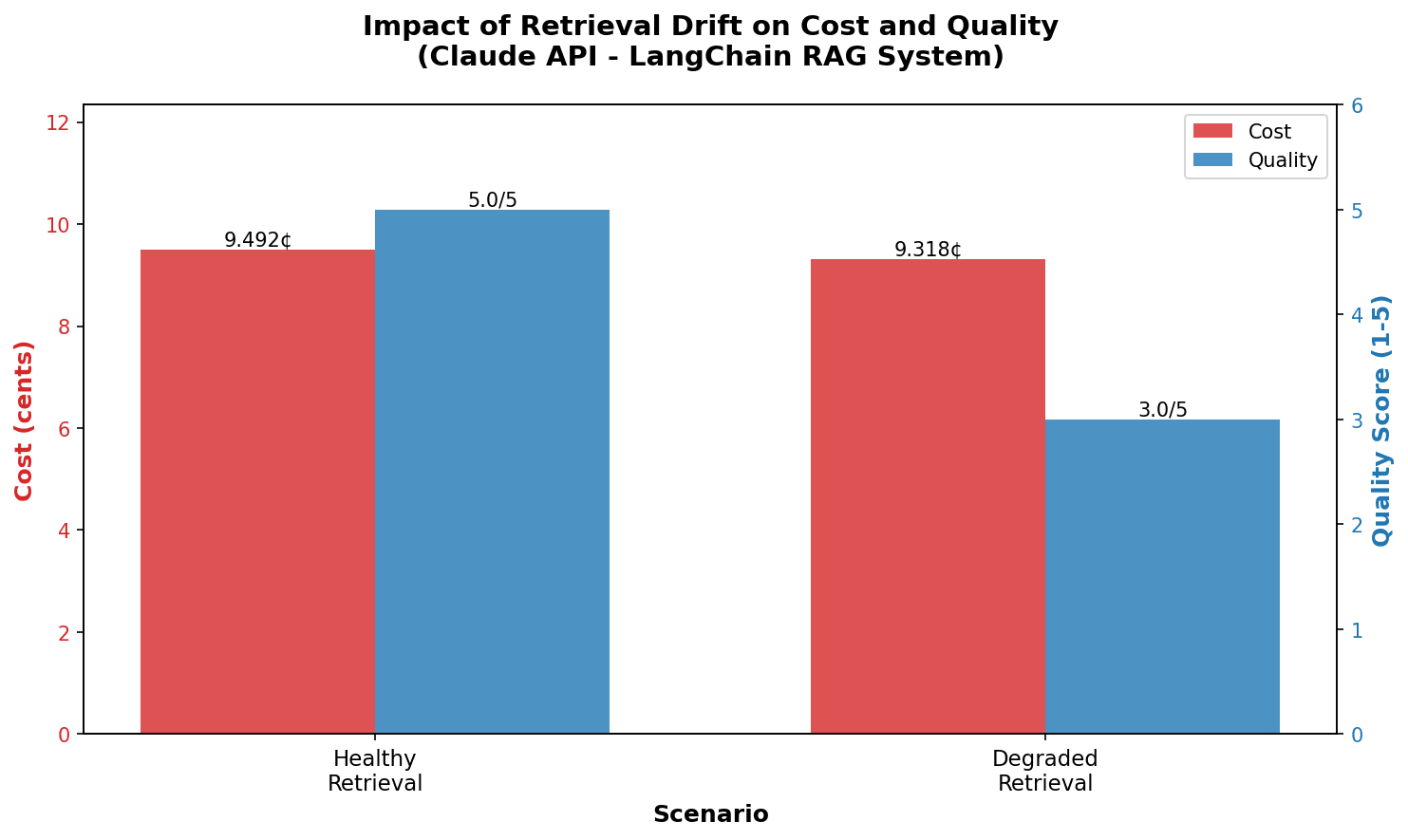
Figure 2: from the Weights & Biases dashboard: Quality degradation from retrieval drift in a LangChain RAG system. While costs remained relatively stable, response quality dropped 40% when outdated documentation entered the retrieval pool.
This experiment powerfully demonstrates a broader, more critical principle for monitoring LLM systems. Aggregate metrics (like overall quality scores, average latency, or cost per query) are crucial. They tell you something is wrong. However, it’s the component-level traces that tell you what is wrong and where to look.
Consider the ripple effects. A 28% increase in input tokens might eventually trigger a cost alert, but only after your system has processed thousands of degraded, more expensive queries. A quality drop from 5 to 3 will show up in user satisfaction scores, but only after users have received incorrect information, experienced frustration, and potentially formed negative impressions. The trace, however, shows an outdated document with an anomalously high relevance score, giving you that critical signal immediately on the very first degraded query.
Effective production monitoring for LLMs absolutely needs both layers:
Without traces, you’re essentially debugging with incomplete information, sifting through symptoms with limited visibility into root causes. With traces, you can move directly from symptoms to the precise root cause, enabling much faster, more targeted interventions.
The powerful principles we’ve discussed (trace logging during inference, automated evaluation on logged data, and visual monitoring for pattern detection) demand robust infrastructure. While you could build a custom solution, modern LLMOps platforms are designed to provide these capabilities out of the box. This section will walk through a practical implementation using W&B Weave, though similar workflows apply to other platforms like LangSmith, Langfuse, or custom solutions.
Production monitoring begins with structured logging that captures component-level data at every step. Each request needs instrumentation to track inputs, outputs, latency, and costs. Here’s how this looks in practice using W&B Weave’s elegant decorators:
import weave
import numpy as np
from anthropic import Anthropic

# Initialize tracking for your project
weave.init('llm-drift-monitoring-tutorial')

# Initialize your Anthropic client
claude_client = Anthropic()

def calculate_cost(usage):
    """Calculate cost for Claude Sonnet 4
    $3/M input tokens, $15/M output tokens"""
    input_cost = (usage.input_tokens / 1_000_000) * 3
    output_cost = (usage.output_tokens / 1_000_000) * 15
    return input_cost + output_cost

@weave.op()
def retrieve_documents(query: str, doc_pool: list, k: int = 3):
    """Retrieval step automatically logged with inputs/outputs"""
    embeddings = get_embeddings([query] + doc_pool)
    similarities = calculate_similarity(embeddings[0], embeddings[1:])
    top_docs = get_top_k(doc_pool, similarities, k)

    return {
        "docs": top_docs,
        "relevance_scores": similarities[:k],
        "avg_relevance": np.mean(similarities[:k])
    }

@weave.op()
def generate_response(query: str, context: str):
    """Generation step automatically logged with token counts and cost"""
    response = claude_client.messages.create(
        model="claude-sonnet-4-20250514",
        max_tokens=1024,
        temperature=0,
        messages=[{
            "role": "user",
            "content": f"Context: {context}\n\nQuery: {query}"
        }]
    )

    return {
        "response": response.content[0].text,
        "input_tokens": response.usage.input_tokens,
        "output_tokens": response.usage.output_tokens,
        "cost": calculate_cost(response.usage)
    }

@weave.op()
def rag_pipeline(query: str, doc_pool: list):
    """End to end pipeline creates a nested trace"""
    retrieval = retrieve_documents(query, doc_pool)
    context = "\n\n".join(retrieval["docs"])
    result = generate_response(query, context)

    return {
        "response": result["response"],
        "metrics": {
            "retrieval_relevance": retrieval["avg_relevance"],
            "input_tokens": result["input_tokens"],
            "output_tokens": result["output_tokens"],
            "cost": result["cost"]
        }
    }
The magic here is the @weave.op() decorator. It automatically logs every function call with its full context: inputs, outputs, execution time, and creates a trace showing the nested operation hierarchy. Token counts are extracted directly from the Anthropic API response objects (response.usage.input_tokens and response.usage.output_tokens). Costs are calculated using Anthropic’s published pricing ($3 per million input tokens and $15 per million output tokens for Claude Sonnet 4).
For the drift simulation in this example, we ran identical queries with different document pools each “day,” manually setting timestamps to create the temporal separation visible in the monitoring charts. This compressed timeline effectively demonstrates drift patterns that would typically emerge over weeks or months in real production systems.
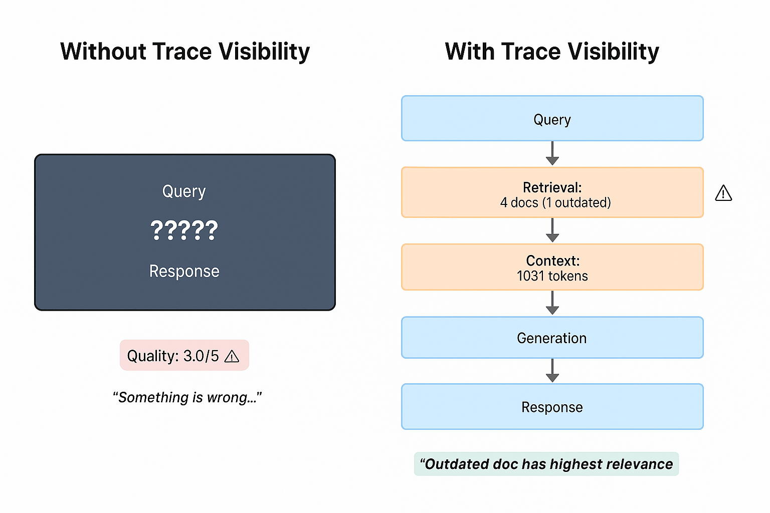
“Figure 3: Trace visibility transforms debugging from guessing (left) to diagnosis (right). Component-level inspection reveals the outdated document causing quality degradation.”
Running your LangChain experiment with Weave instrumentation produces detailed traces for every single query. The W&B trace view provides an incredibly granular look at the exact execution flow: the rag_pipeline call triggers retrieve_documents, which returns specific documents with their relevance scores. This then feeds into generate_response, which consumes those documents and returns an LLM response along with token counts and calculated cost.
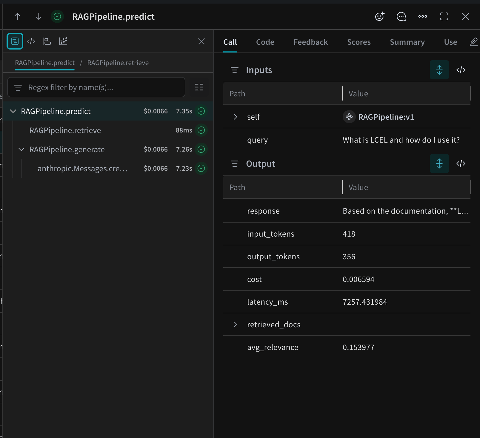
Figure 4: Component-level trace showing nested operations (retrieve then generate) with metrics at each step. This query used 418 input tokens and 356 output tokens, with an average retrieval relevance of 0.154.
The trace detail in the image reveals a wealth of information invisible to aggregate metrics. You can see precisely which documents were retrieved, their individual relevance scores, how many tokens the context consumed, and how long each step took. When quality degrades, you can immediately drill into the trace and identify the problematic document that caused the issue, or pinpoint a slow-performing step.
This capability directly matches what we observed in our drift experiment. We saw that an outdated LangChain documentation page had a higher relevance score than current, accurate documents, leading the retrieval system to prefer it. Without this level of trace visibility, the problem would manifest as a mysterious, hard-to-debug drop in quality. With traces, you can see the root cause in the very first degraded query, enabling swift action.
Weave automatically aggregates these individual traces into meaningful time series metrics. The platform continuously tracks costs, latency, token consumption, and any custom metrics you define (like retrieval relevance) across all queries. This forms the crucial continuous-monitoring layer, designed to surface drift in real time.
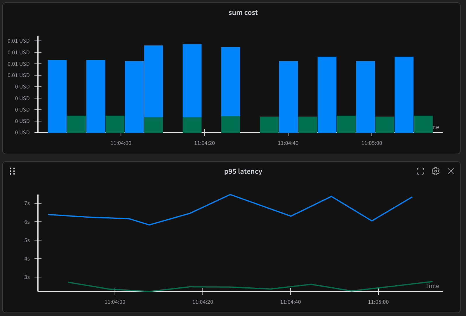
Figure 5: Real-time cost and latency trends. The cost chart shows per-request spending over time, while p95 latency reveals performance patterns
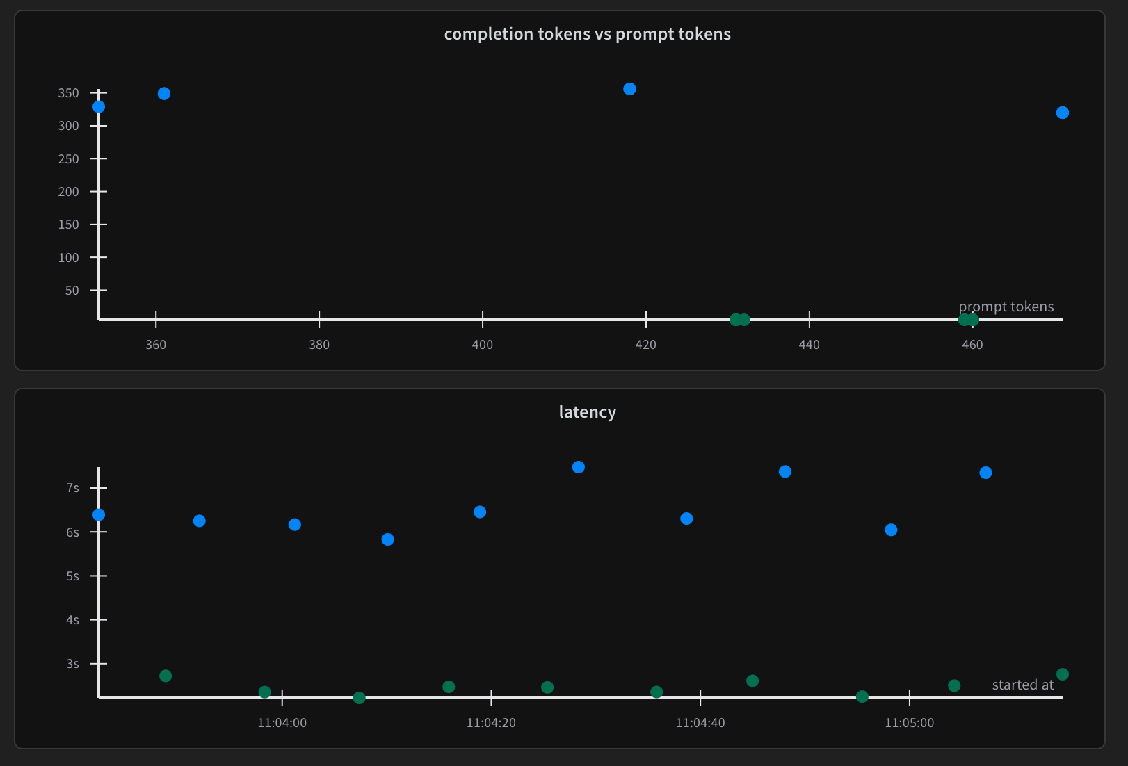
Figure 6: Token consumption patterns showing the distribution of prompts versus completions. Each point is a query that shows how context size correlates with response length.
These interactive dashboards provide a real-time pulse on your system’s health. The “completion tokens vs prompt tokens” chart shows the relationship between the size of the context provided to the LLM (prompt tokens) and the length of its response (completion tokens) across all queries. Each dot represents a single query.
This view is incredibly powerful for surfacing retrieval drift through unexpected token patterns. If your typical queries usually consume between 350 to 450 prompt tokens, but you suddenly see clusters appearing at 450 to 470, it’s a strong indicator that your retrieval system is pulling more context than usual. This often happens before quality metrics overtly degrade. The system is simply working harder (and potentially incurring higher costs and higher latency) to maintain the same output quality.
The latency chart shows the distribution of execution times for your LLM calls. Most queries might complete consistently within 6 to 7 seconds. However, any outliers exceeding 7 seconds clearly indicate either exceptionally complex queries, potential system performance bottlenecks, or an LLM behaving unexpectedly. These are all signals worth investigating to maintain a smooth user experience.
Running our three-day drift simulation with Weave instrumentation produced concrete results visible in these monitoring dashboards:
Day 1 (Healthy baseline):
Day 2 (Introducing noise/early drift):
Day 3 (Full degradation):
Notice something critical here: the quality scores remained stable at 4.0 across all three days. On the surface, this might lead you to believe the system is perfectly healthy. However, the monitoring dashboard immediately reveals the truth: token consumption increased by 12% and average retrieval relevance dropped by 3%. These are crucial early warning signals, visible in the monitoring dashboard before your primary quality metrics or, more importantly, your users, even begin to show problems.
This demonstrates a key insight: cost and efficiency drift often precede quality drift. By the time user satisfaction drops due to declining quality, you may have already processed thousands of queries at an inflated cost. Monitoring these component-level metrics and their distributions catches these issues much earlier in the degradation curve.
Weave seamlessly connects monitoring to evaluation through its powerful Evaluation API. This allows you to automatically score recent production data and continuously track quality trends over time:
import weave

@weave.op()
def judge_quality(query: str, response: str):
    """LLM as judge scorer for automated evaluation"""
    score = judge_llm.invoke(
        f"Rate this response's accuracy, helpfulness, and coherence "
        f"on a scale of 1 to 5 for the query '{query}': {response}. "
        f"Return ONLY a single number between 1 and 5, nothing else."
    )

    try:
        return {"quality_score": int(score.strip())}
    except ValueError:
        return {"quality_score": 0}

# Recent queries from your production logs in W&B
recent_queries_sample = [
    {"query": "How to do X in LangChain?", "response": "Response for X"},
    {"query": "Explain Y in Python.", "response": "Response for Y"},
    # ... up to 100 recent production queries
]

# Set up the evaluation
evaluation = weave.Evaluation(
    dataset=recent_queries_sample,
    scorers=[judge_quality]
)

# Run the evaluation against your pipeline
results = evaluation.evaluate(rag_pipeline)

print("Evaluation results available in W&B.")
This code creates a continuous feedback loop: production traffic gets logged, recent queries are automatically evaluated, quality trends are monitored, and any anomalies trigger immediate investigation. The entire workflow remains within a single platform, eliminating the need to jump between disconnected logging infrastructure, bespoke evaluation scripts, and disparate monitoring dashboards. This streamlined approach significantly reduces context switching and accelerates the debugging process.